Amortization Schedule in Excel

Have you ever wondered how the monthly loan payment breaks down components like interest, principal and the like? 

The answer is simple: Amortization calculator. 

This is a specific kind of financial tool gives you a detailed breakdown of loan calculations. Fully understanding loan payment can be tricky. On top of that, financial jargons like ‘interests’, ‘principals’, or even ‘amortization’ can go unexplained, leaving you in doubt about where your earned money is going.

Therefore, based on my knowledge gained from years of using this tool, I have curated this detailed guide on the amortization table in Excel.

What Is The Amortization Schedule?

In general, the Amortization table and scheduling method is crucial for students with accounting courses. The main concept behind the amortization schedule is a table formation that assists in breaking down the loan payments on a fixed rate. 

Car loans and mortgages fall under these loan processes. The loan amortization schedule in Excel helps to get a detailed and clear idea about the loan payment. It shows the exact amount of your payment for interest and the amount that is applied to reduce the principal amount (this is the amount that you borrowed). 

As time passes with the consistency of the payments, the principal amount starts to increase, while the amount in the interest section starts to decrease. This decrease in interest shows the decline of loan payment as you continue to pay it.

The detailed breakdown through the Excel loan payment schedule gives you a detailed idea about how much from your total earnings are going towards reducing your debt. The table also indicates the amount is going towards the interest rates.

Loan Amortization

Amortization is the procedure of paying off a certain amount of debt within a tentaive deadline in regular instalments for both interest and principal. In this case, the loan is supposed to be repaid by a given maturity date. 

The loan amortization schedule in Excel helps to represent the principal amount as well as the interest amount comprising all the levels until the loan is paid off at the end of its term. In this procedure, a portion of a high percentage of the monthly payment goes to the interest during the loan process. On the other hand, a maximum amount is added to the loan principal along with the following order of payment.

The amortization schedule is mostly calculated with the help of potential financial calculators, and various spreadsheet packages such as Microsoft Excel. These schedules are customisable based on how much loan is taken by the borrower as well as personal circumstances. Amortization calculators also allow you to advance the process for loan payments.   

Formulas For Calculating Loan Amortization

Amortization formulas are handy for creating a loan amortization table, offering a clear breakdown of interest and principal for easy loan payment calculations in Excel. The key formulas include:

• Principal Payment Formula:

Principal payment = Total Monthly Payment (TMP) - Outstanding Loan Balance (OLB)

• Monthly Payment Estimation:

To estimate monthly payments or compare loan options based on factors like loan amount and interest rate, use:

Monthly Payment (TMP) = [i * (1 + i)^n] / [(1 + i)^n - 1]

Where:

• i: The monthly interest rate is found by dividing the annual interest rate by 12.
• n: The total number of payments is calculated by multiplying the number of years for the loan by 12.

For instance, if your annual interest rate is 5%, the monthly interest rate would be approximately 0.41%. Similarly, if you have a 12-year loan, you'll make a total of 144 payments. These formulas simplify the process of understanding and calculating loan payments.

How to Set Up a Loan Amortization Table

Now, let’s learn how to create an amortization chart to understand the procedure better. 

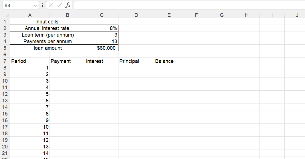
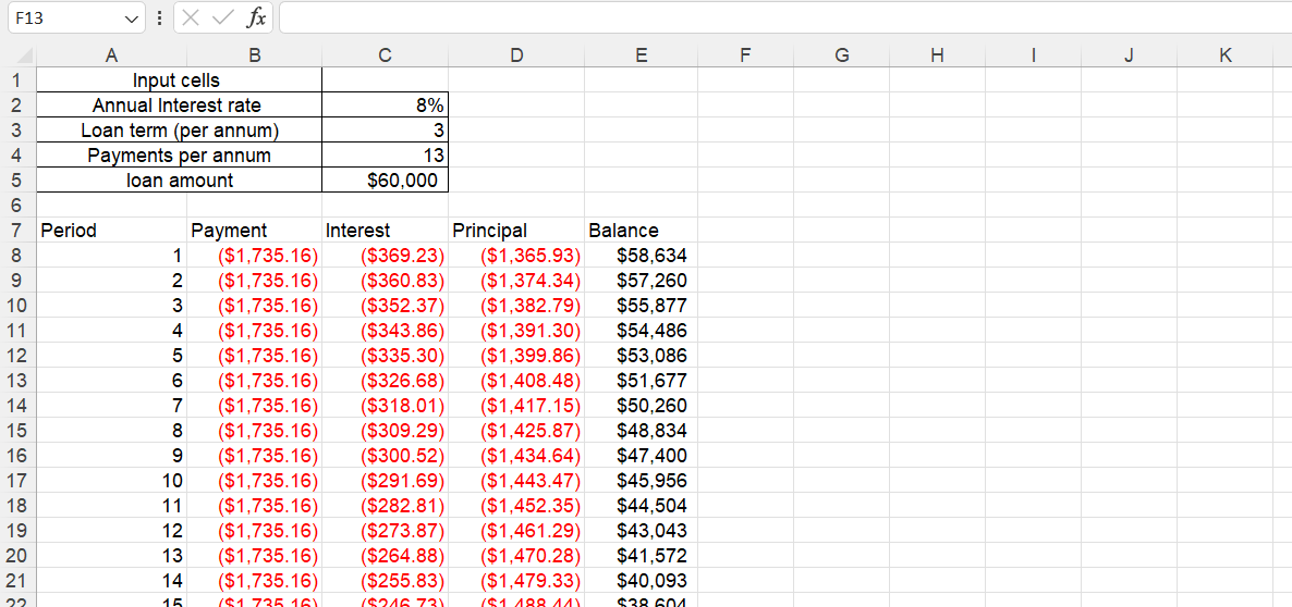
Step 1: Setting up the amortization table

To start with the amortization table, first, you need to enter all required components of the loan payment. Such as:

●       The annual interest rate will go into C2

●       Loan term years will go in C3

●       The number of payments per annum will go into C4

●       The amount of loan taken will go in C5.

After creating the above chart, now you need to create the amortization table where you need to put a period, payments, interest rate, principal and balance from A7 to E7. After that, enter a series of numbers (from 1 to 39, for this example) which is equal to the total payment number in the period column.

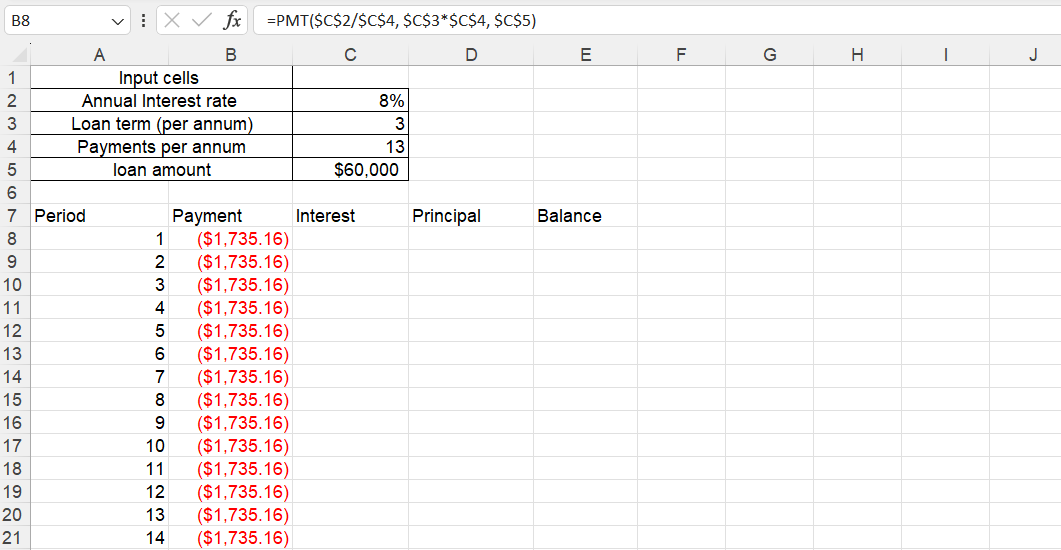
Step 2: Calculation for the total payment amount (PMT function)

For the calculation of the total payment amount, you need to use the PMT function which includes rate, nper, pv, [fv], and [type]. Now to manage different types of payment frequencies appropriately, consistency is the ultimate key. One needs to maintain better consistency while putting values for rate and nper arguments.

●       Rate: to obtain the rate, you can divide the annual interest rate by the number of payment periods per annum. The formula is ($C$2/$C$4).

●       Nper: to obtain the value of nper, the payment period per annum needs to be multiplied by the number of years. The formula is ($C$3*$C$4).

●       pv: for this particular argument, you can enter the loan amount. The syntax for pv is ($C$5).

●       As for fv and type, they can be left out as they carry a default value which does not take an active part in the process.

After putting all the arguments, we get the following formula:

=PMT($C$2/$C$4, $C$3*$C$4, $C$5).

This formula will go into the cell B8. please note that you need to put the formula in an absolute cell that is referred to here. Once you put the formula in B8, drag the column down to achieve the same payment amounts for all periods. 

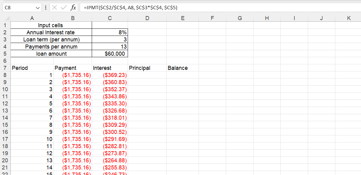
Step 3: calculation of interest function

To find out the value of the interest of the loan payment, the IPMT formula is used which is:

=IPMT($C$2/$C$4, A8, $C$3*$C$4, $C$5)

Here, the arguments are similar to the arguments included in the PMT function. However, in this case, a relative cell reference, A8 is included as the interest value is supposed to change by the time of periods of loan payment.

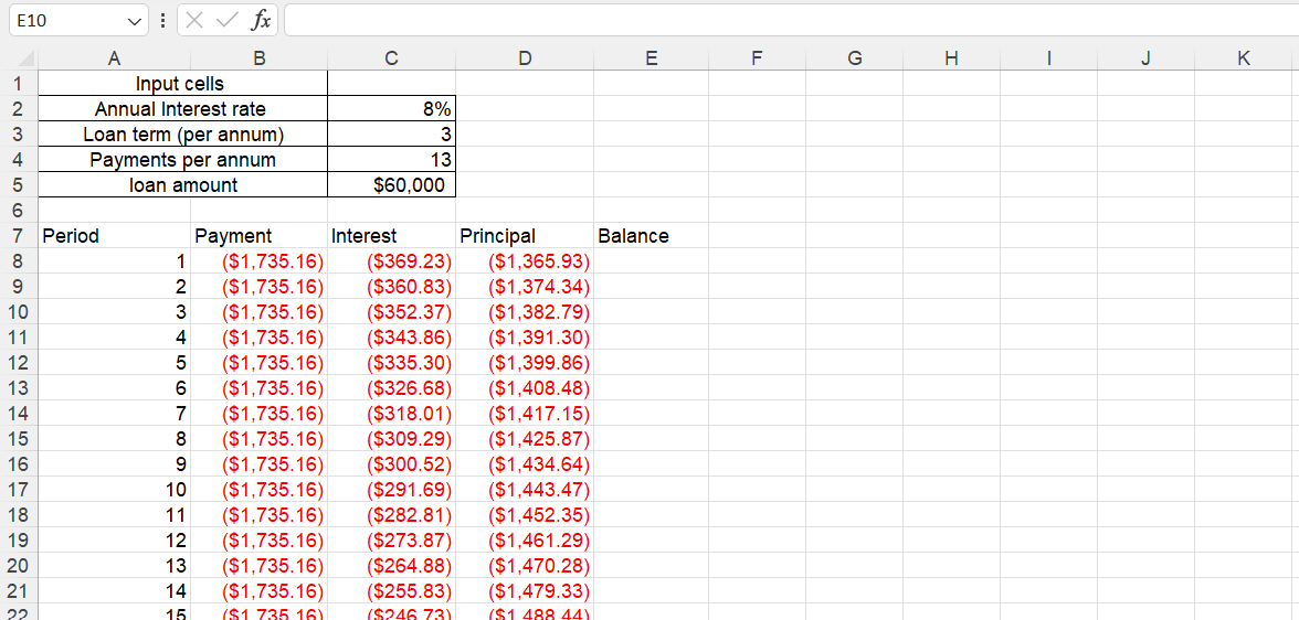
Step 4: calculation of principal function (PPMT function)

To continue with the calculation of the principal function, you need to enter the formula: =PPMT(I/Y, Period, Nper, PV, [FV], [Type]) in the principal column in D7. 

In this case, all the formulas are the same as IPMT functions. Similar to the calculation of interest rate, you will need to add the period of payments to achieve the principal amount values. So the formula will go like this:

=PPMT($C$2/$C$4, A8, $C$3*$C$4, $C$5)

Step 5: calculating the remaining balance value

To find out the remaining balance in the amortization table in Excel, you need to enter two different formulas. Firstly, for the first payment in the E8 cell, the C5 value which is the loan amount and the D8 value, the first period for payment will be added. The formula will be:

=C5+D8

After the first balance, the second balance will be calculated by adding up the previous balance value in E8 with the present principal in D9. This applies for the rest of the period payment until the month 39th (for this example). The formula is:

=E8+D9

So, this is how you can easily calculate the Excel loan repayment schedule by simple formulas to develop the amortization table. 

Why Is Amortization Useful?

The amortization table in Excel has various useful purposes that make the loan repayment process easier for the borrowers. I’ve listed a few advantages of this Excel feature that proved quite beneficial in my endeavors:

1. Comparison and Assessment: The amortization table is useful for making a comparison between loan offers as well as assessing the borrowing costs. 
2. Analysis of Interest Payments: This table helps in analyzing the due amount of the interest payment and identifying various favourable terms.
3.  Cash Flow Management: This table helps in managing cash flow management by the proper breakdown of one’s loan payment. The breakdown is also useful in managing the budget from your earnings.
4. Early Payment Planning: A mortgage amortization schedule is useful to pay down your mortgage principal in a short time with less interest rate involved. This is how you can opt for early payment planning for your mortgages and loans.
5. Negotiation Tool: With a proper amortization table in Excel, the borrowers can make an easy approach to the lenders with an easy understanding and breakdown of the loan payment. This helps them to make proper negotiations on good terms.

In Summary

Crafting a loan repayment schedule is easiest via the amortization table in Excel. Now that we have summed up this tutorial, I hope it empowers you to learn about the table to track down your loan progress in future. 

You can also find an online free amortization schedule calculator to undertake easier steps for your loan repayment planning. In addition to this, there are several advanced Excel courses you can opt for from UpGrad to master more Excel skills and financial analysis. 

Frequently Asked Questions

1. How do I create an amortization schedule in Excel?

You can use the PMT formula in Excel to calculate the payment properly. For both principal and interest payments, you can use the PPMT and IPMT formulas respectively.

2. How to do an Amortization schedule?

The amortization schedule can be created by calculating the interest portion and principal portion for every single payment over the term.

3. How do I calculate monthly payments in Excel?

You can use the formula for the PMT function: =PMT(rate/12, nper, pv) for your monthly payment calculations.

4. What is schedule amortization?

The schedule amortization is known as a table that assists you in breaking down the loan into interest and principal that needs to be paid off over the loan terms.

5. How do I calculate loan amortization in Excel?

You can calculate the loan amortization by using the PMT function in Excel.

6. What is the formula for amortization of a loan?

There is no specific formula for the amortization table, thus, you can use the following:

• PMT function: =PMT(rate/12, nper, pv)
• IPMT function: =IPMT(rate, per, nper, pv, [fv], [type])
• PPMT function: =PPMT(rate, per, nper, pv, [fv], [type])
  

7. How do I prepare a loan amortization schedule?

You can list down the periodic payments along with the breakdown of principal and interest values as per the loan term, to prepare the loan amortization schedule.

8. What is the formula for loan in Excel?

The formula for calculating loan in excel is: =PMT(rate/12, nper, -pv)