Columns in Excel

Without Excel, working with large datasets can be very hectic and overwhelming. Excel allows me to organize the data in a compact manner. This simplifies my work to a great extent.

Columns are the vertical divisions extending from left to right of the spreadsheet. There are also horizontal divisions known as rows, traversing the sheet from top to bottom. This framework of rows and columns facilitates data entry, visualization, and analysis.

Let us explore columns in Excel and its various operations.

What are Rows and Columns in Excel?

Datasets in Excel are represented in a tabular format. This format consists of horizontal rows and vertical columns.

Rows in Excel

Rows are groups of horizontal cells appearing from left to right in the spreadsheet. Each row is represented with a number starting from 1, 2, 3… and so on.

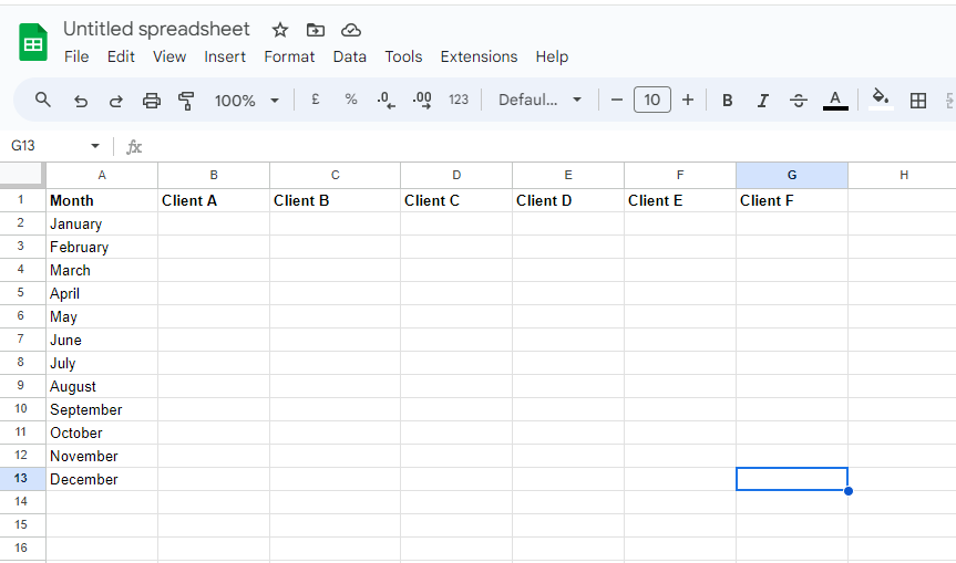
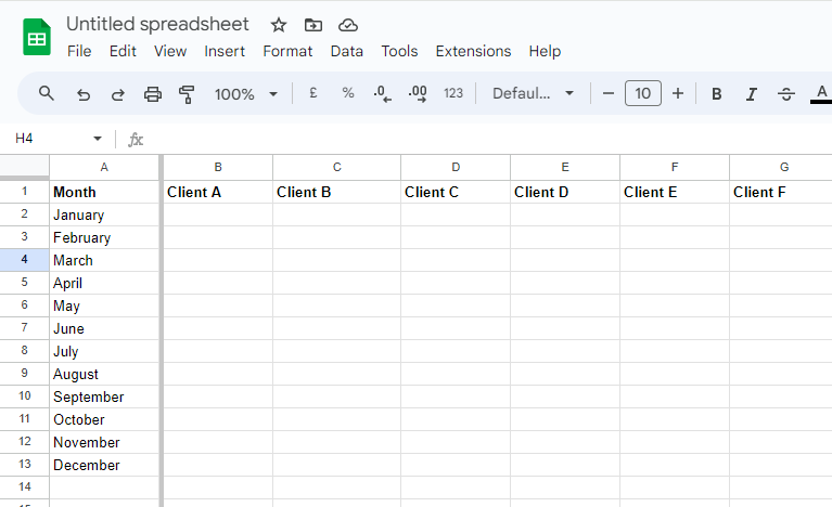
Columns in Excel

Columns are the vertical groups of cells present on a spreadsheet. Each of these columns is named after a letter and they run top to bottom in an Excel spreadsheet.

As we can see in the image, the column name starts from A, B, C… and so on up to Z. After which comes columns AA, AB, AC… and continues till the last column - XFD.

Operations in Excel using columns

Using Excel for sorting data has been life-changing for me. Many operations can be performed using Excel which makes the tedious process of sorting and analyzing data a much easier job.

Here are some operations that you can perform using Excel columns:

1. Comparing columns in Excel

Comparison between two columns of Excel can be done in several ways. Some of these ways are as follows:

Case 1: Comparison with the equals operator

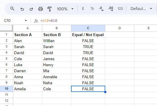
Comparing two columns in Excel can be done row by row using the equals operator. To use this operator, you will have to use the syntax: = 1st cell name = 2nd cell name. This will only give you the result for those two particular cells.

However, if you want to compare all the data, you simply have to drag your cursor to the range that you want. If it matches, the result will be ‘True’ or else ‘False’

In the example given above, data in columns A and B can be compared using this operator. The syntax I have used in this scenario is =A2=B2 and adjusted the cursor to the desired range.

Case 2: Comparison with the IF condition

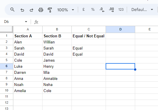
The IF condition can also be used for comparing two columns in Excel. The syntax used in this example to compare columns A and B is =IF(A2=B2,”Equal”,””). It returns ‘Equal’ against rows containing matching values and the remaining rows are left empty.

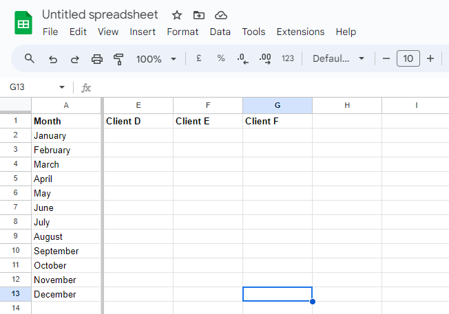
2. Freezing columns in Excel

If you want a particular column visible while navigating through the other parts of the sheet, you can freeze columns in Excel. It is very simple and does not require any syntax to perform.

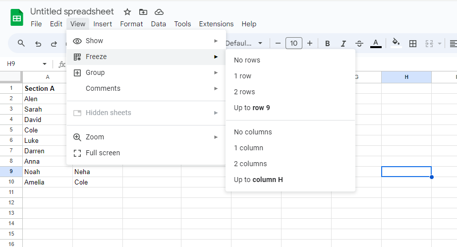
If you want to freeze columns in Excel, follow the given steps:

• Step 1: Place your mouse on and click on the ‘View’ tab.
• Step 2: Select the ‘Freeze’ option.
• Step 3: From the drop-down menu you can choose how many columns (or rows) you want to freeze.

Note: In the example used, I have placed the cursor on column H. which is why the option for freezing is available till column H for me. You can place your cursor on the column till which you want to be frozen, and the option will appear accordingly.

This feature comes in very handy when I want to navigate through my annual sales record. I simply freeze the first columns and move through the sheet. This can be better understood by the example given below.

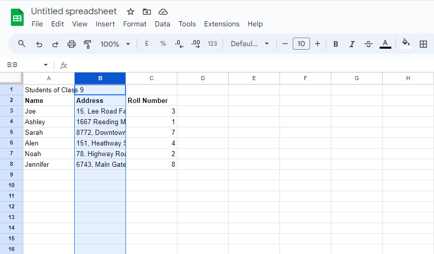
3. Hiding columns in Excel

If there are columns that you might not require immediately, you can choose to hide columns in Excel. To hide a column, select the column you want to hide, right-click on it, and then click on ‘Hide’.

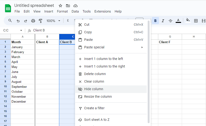
Once you have hidden the column of your choice, the position of the hidden column will be marked with two arrowheads.

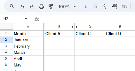
4. Unhiding columns in Excel

By selecting the two columns around the hidden one, you can unhide columns in Excel. After selecting, right-click and choose the ‘Unhide’ option.

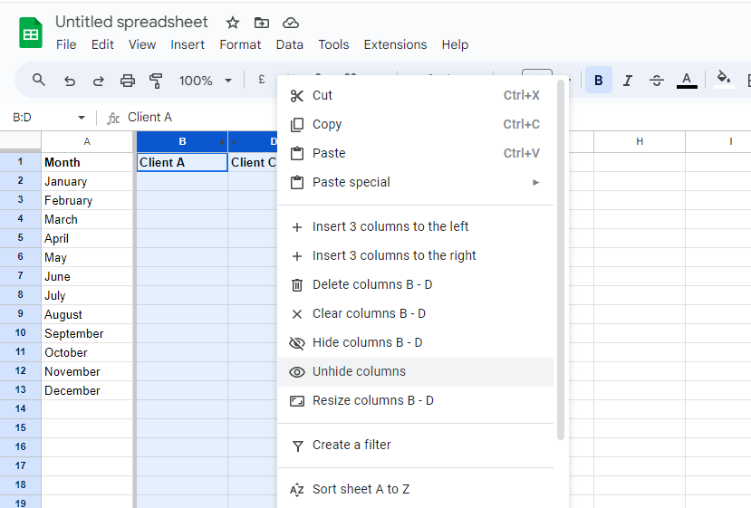
Now, the hidden column will be visible.

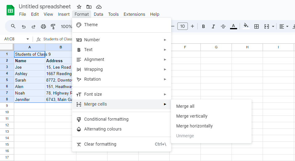
5. Merging two columns in Excel

When you want to combine the content of two or more cells into a single one, merging the cells is a great idea. I have used this for creating a title that contained multiple columns. It combined the data into a single cell for easier understanding.

To merge columns in Excel, highlight the columns that you want to merge and click on the format option. From the drop-down menu click on the ‘Merge’ option and choose what kind of merging you want.

6. Adjusting column width in Excel

Every column on the spreadsheet has the same width. This can sometimes be a disadvantage as all the content in those cells is not visible. The column width can be adjusted for better visibility and analysis.

The Excel column width can be adjusted in the following way.

• Step 1: Position your cursor over the column line on its heading. The cursor becomes a double arrow.
• Step 2: Drag your mouse to adjust the column width.
• Step 3: Release mouse mouse and the column width will be adjusted.

Another way to adjust Excel column width is to place your cursor on the column line and double-tap on it. This automatically changes the width of the column to fit in the content.

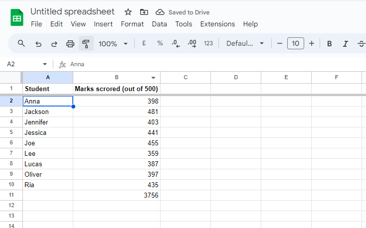
7. Excel column total

This feature has been a lifesaver for me. It helps me calculate the Excel column sum within seconds. It can be done using the syntax: =SUM(Starting cell: Last cell).

Let us see an example.

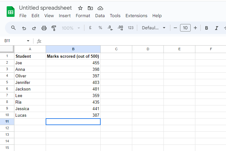
If I want to find the sum of marks scored by all students, I will use the syntax: =SUM (B2:B10).

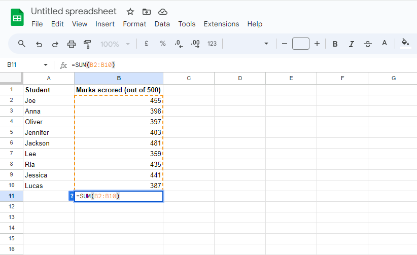
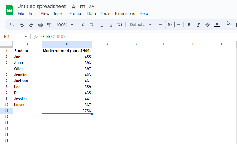
On pressing Enter, the sum will be calculated.

This is one of the operations you can use in Excel. Check out more formulas in Excel to perform other functions.

8. Sorting Excel column

Are you struggling to find data in your Excel sheet? Using Excel column sorting to search and find data easily. Having the data sorted alphabetically makes it easier to find what you are looking for.

Check out the previously used example where the names of the students are present in a disoriented manner.

To sort the names alphabetically, you should first freeze the heading row. After which take your cursor to the first cell of the column, and choose the ‘Sort sheet’ option from ‘Data’. You get to choose how you want your column sorted.

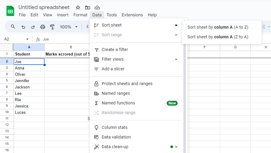
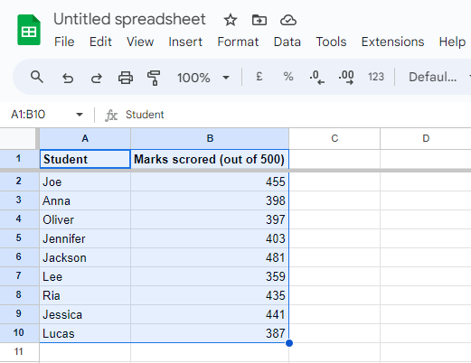
Finally, the sheet will look like this. All the column contents in column A have been arranged from A to Z.

What is an Excel Chart?

An Excel column chart is used for visually representing the data, making it easier to compare values across categories. If I had to analyze the marks of my students, this is one of the best ways to do so.

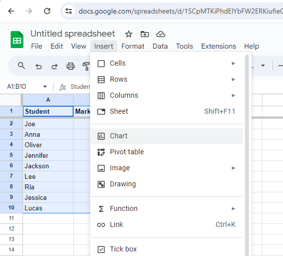
How to Build One

To create a column chart, follow the given steps:

• Step 1: Click and drag your mouse across the data range that you want to create a chart for.

• Step 2: Click on ‘Insert’ and select the ‘Chart’ option from the menu.

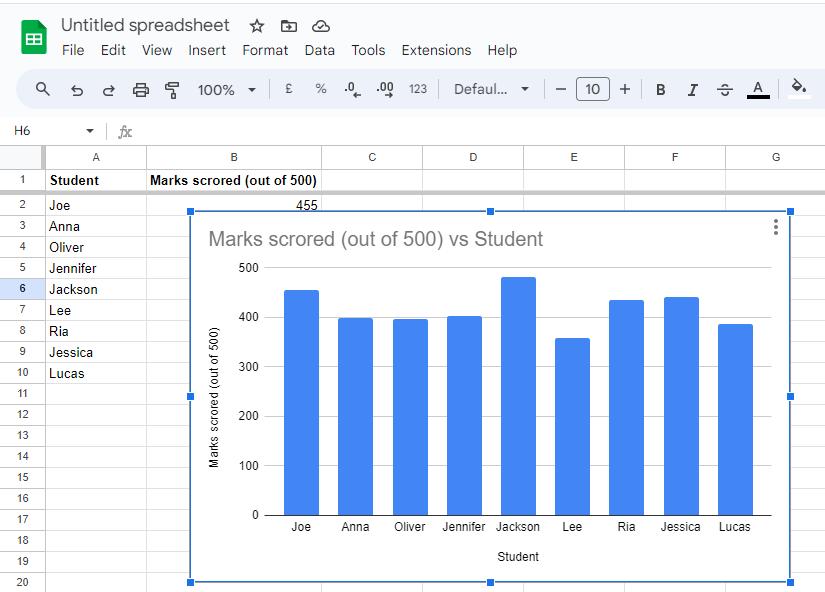
On selecting ‘Chart’ from the drop-down menu, you will be provided with the chart in a bar graph format.

This has helped me easily calculate the range of a data set while visually analyzing it.

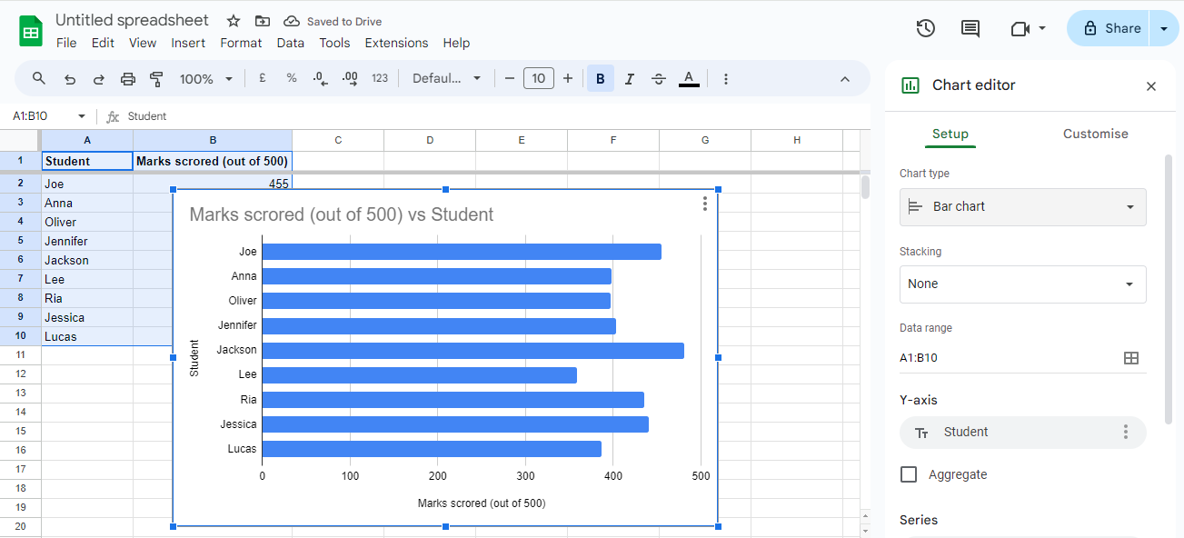
You can also customize the chart according to your liking from the ‘Edit’ option given on the right-hand side of the screen.

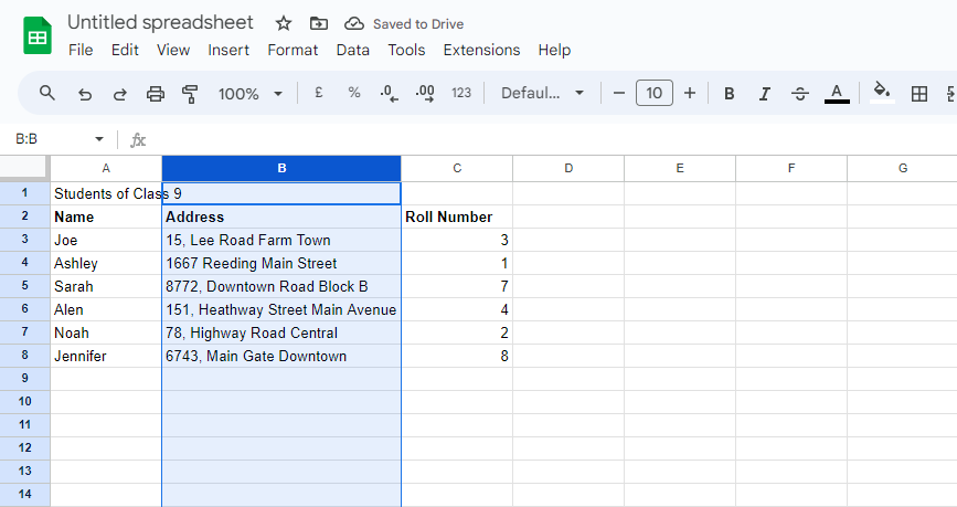
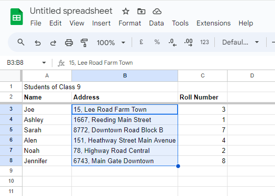
How to Split Text in Columns?

Clearly defined data, separated by a comma (generally) can be split into different columns. It can be done by following the given steps:

• Step 1: Place and drag your mouse over the column that you want to split.

• Step 2: Click on ‘Data’ and choose the ‘Split text to columns’ option.

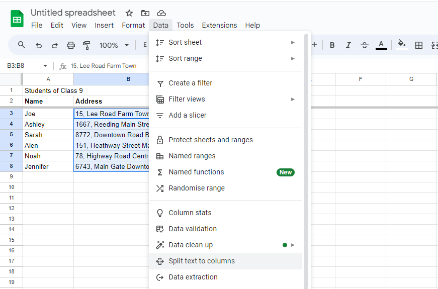
• Step 3: Press enter and the column will be sorted according to commas.

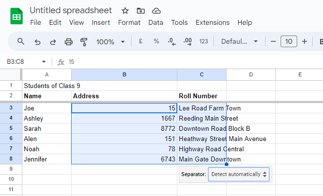
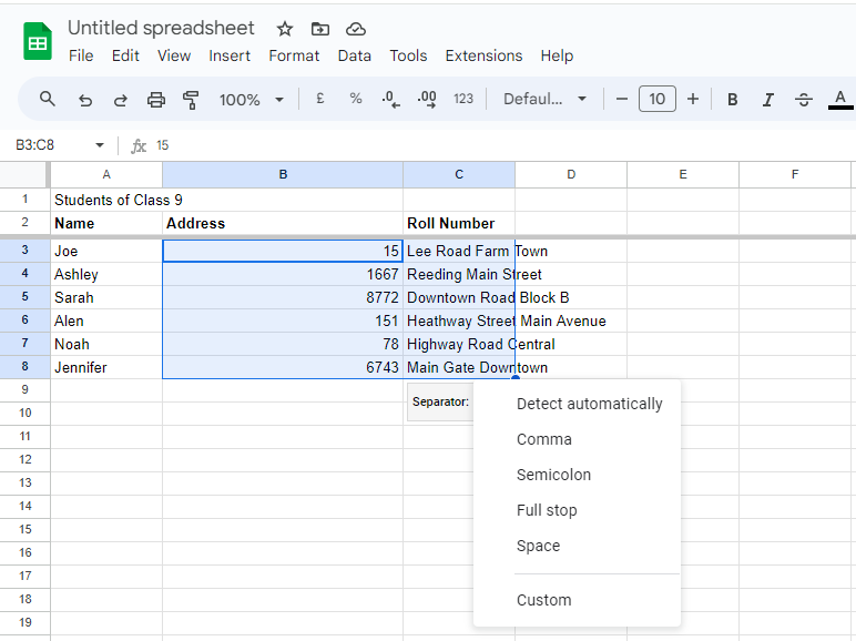
This can however be customized. You can choose to split the column by spaces, full stop, or semi-colon. It can be selected from the option provided.

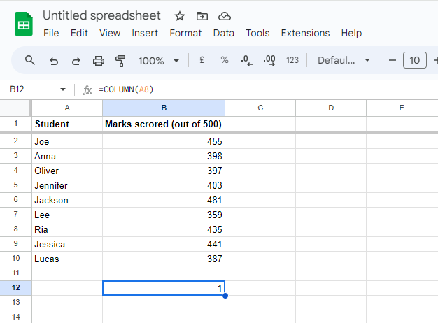
The COLUMN Function in Excel

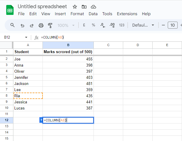
It is a reference or lookup function that searches and provides the column number of the given reference cell. The syntax used for this function is: =COLUMN([reference cell]).

For instance, in the example given here, if I want to find the column number of cell A8, I will simply use the syntax: =COLUMN(A8). The column number will be provided in the cell where the cursor has been placed.

Why is Data Formatting Necessary?

Formatting column data makes it appear more visible especially when there is a large worksheet. I always tend to alter the default formats of a worksheet like changing the font size, style, color, or alignment. This helps me identify the important data when browsing an extensive spreadsheet.

As the image given shows, there are many options for formatting the content of a cell.

Final Words

When dealing with large datasets, Excel can serve as a blessing. It helps in organizing the data, which facilitates superior data analysis and visualization. Excel spreadsheets are used for manipulating stored data using columns in Excel commands.

Using Excel will help you make your work life smoother and grow in your career. Excel proficiency is needed in several fields. You can boost your skills with the certified courses offered by upGrad.

Frequently Asked Questions

1. How many columns are there in Excel?

There are 16,384 columns in Excel.

2. What is row and column?

Rows are horizontally arranged series of cells. Whereas columns are vertically arranged groups of cells.

3. What is the column operation in Excel?

The COLUMN function returns the column number of a given cell.

4. What is column format in Excel?

Excel uses a general format for all its content. However, this can be changed by altering the size, font, or color of the text.

5. What is column to text in Excel?

The text to column button is present in the Data tab in the Data tools group.

6. What is column data format?

The column data format in Excel specifies how the column values are displayed in stories, dashboards, reports, etc.