Count Colored Cells in Excel

As a child, I was fond of using colored sketch pens in my notebook. Even now that I work on MS Excel as an adult, I find it easier to sort and store data using colors, which makes the data sheet easier on the eye.

In Excel, ‘count cells with specific color’ option is also available.

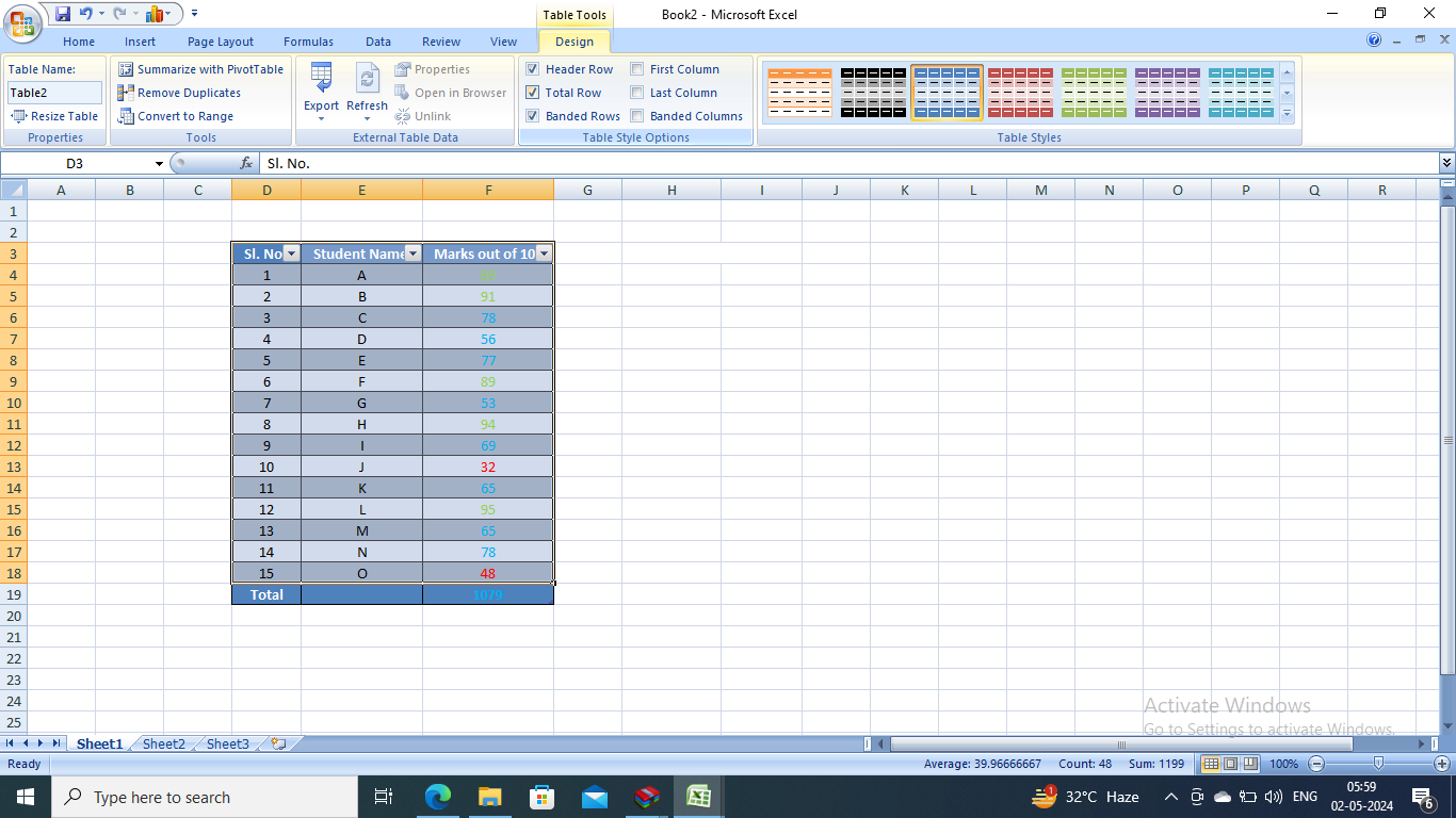
For example, we prepared a sheet that contained the marks of 15 students in Mathematics. All the marks above 80 have been flagged green, those between 50 and 80 have been flagged yellow, and those below 50 have been flagged red.

Although it is easy to keep a count of these manually in case of small data sets, it becomes a nerve-wracking task for sheets that contain humongous amounts of data.

I have figured out a few ways, which I will be sharing in this Excel tutorial today. Stick through till the end to understand how to count colored cells in Excel.

Count Colored Cells in Excel Using VBA

You can count colored cells in Excel by cell color as well as by font color.

Let me first make it clear to you that these functions are not going to be available by default, unlike other functions like Sum, Average, etc. But don’t worry! I have also covered how to add this function to your workbook.

Open an Excel sheet and press “Alt+F11”.

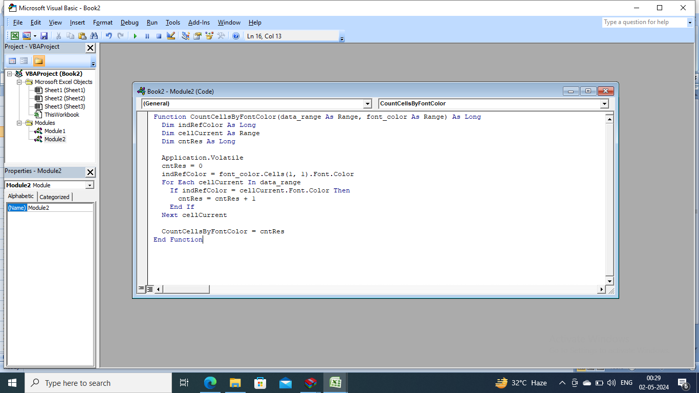
The Microsoft Visual Basic window will appear on the screen. From there, choose “Insert” and select “Module”. There, write the code:

Function CountCellsByMatchingColor(targetRange As Range, referenceColor As Range) As Long
Dim colorToMatch As Long
Dim currentCell As Range
Dim cellCount As Long
' Set the volatile flag to ensure recalculation on changes
Application.Volatile
' Initialize the cell count
cellCount = 0
' Extract the color value from the reference cell
colorToMatch = referenceColor.Cells(1, 1).Interior.Color
' Loop through each cell in the target range
For Each currentCell In targetRange
' Check if the cell's interior color matches the reference color
If currentCell.Interior.Color = colorToMatch Then
cellCount = cellCount + 1 ' Increment the cell count if there's a match
End If
Next currentCell
' Return the final cell count
CountCellsByMatchingColor = cellCount
End Function

Voila! The functions are now added to your Excel workbook.

Counting Cells by Fill Color

Now, prepare a data sheet. I will be using the example that I have cited in the introduction. Next, follow the steps mentioned below:

Step 1: Segregate the data using colors.

Step 2: Use another cell in the sheet close to your table. Insert the colors that you have used in the table. For example, I have used three colors here - green, yellow, and red. I have filled these three colors in the cells H6, H7, and H8.

Step 3: In the cells adjacent to the colored cells, where you want the values to be displayed, insert the formula =CountCellsByColor(Cell range, criteria), where cell range denotes the cells where the data is entered, and criteria denotes the color whose cell count you want to extract.

For example, in the given data sheet, if we want to count the number of green cells, we must use the formula =CountCellsByColor(E6:E20, H6). Drag the formula downwards to apply the same for the other two colors.

The result will appear thus:

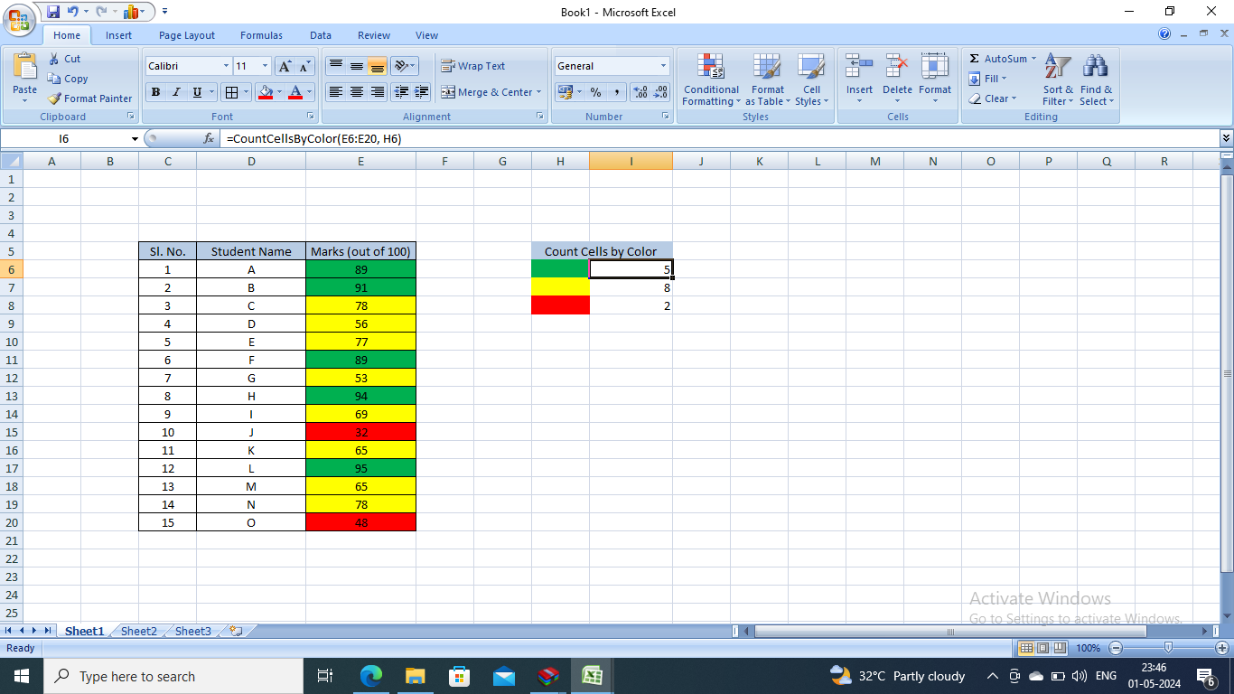
This makes the data easy to comprehend. From the above datasheet, we can decode that 5 students scored above 80, 8 students scored between 50 and 80, and 2 students scored below 50.

Counting Cells by Font Color

To count colored cells in Excel by font color, you will first have to add the function to your workbook. Use the code in the Microsoft Visual Basic:

Function CountCellsByMatchingFontColor(targetRange As Range, referenceColor As Range) As Long
Dim referenceFontColor As Long
Dim currentCell As Range
Dim cellCount As Long
' Set the volatile flag to ensure recalculation on changes
Application.Volatile
' Initialize the cell count
cellCount = 0
' Extract the font color value from the reference cell
referenceFontColor = referenceColor.Cells(1, 1).Font.Color
' Loop through each cell in the target range
For Each currentCell In targetRange
' Check if the cell's font color matches the reference color
If currentCell.Font.Color = referenceFontColor Then
cellCount = cellCount + 1 ' Increment the cell count if there's a match
End If
Next currentCell
' Return the final cell count
CountCellsByMatchingFontColor = cellCount
End Function
Function CountCellsByMatchingFontColor(targetRange As Range, referenceColor As Range) As Long
Dim referenceFontColor As Long
Dim currentCell As Range
Dim cellCount As Long
' Set the volatile flag to ensure recalculation on changes
Application.Volatile
' Initialize the cell count
cellCount = 0
' Extract the font color value from the reference cell
referenceFontColor = referenceColor.Cells(1, 1).Font.Color
' Loop through each cell in the target range
For Each currentCell In targetRange
' Check if the cell's font color matches the reference color
If currentCell.Font.Color = referenceFontColor Then
cellCount = cellCount + 1 ' Increment the cell count if there's a match
End If
Next currentCell
' Return the final cell count
CountCellsByMatchingFontColor = cellCount
End Function

This way, the count cells by font color will be added to your workbook.

Next, open a worksheet and enter the data. I will be using the same dataset as above, the only difference being that instead of filling colors in the cell, I will be using colored fonts.

Follow the steps mentioned below to count colored cells in Excel by font color:

• Step 1: Based on the criteria decided by you, add font colors of your choice. In this example, I have used 3 colors- green, blue, and red.
• Step 2: In an adjacent set of cells, write something and add the same font color as the one you have used in your dataset. Here, I have written Sample 1 in green, Sample 2 in blue, and Sample 3 in red.
• Step 3: To count the number of cells whose content is written in green, go to the next empty cell where you want the result to be displayed and use the Excel count colored cells formula =CountCellsByFontColor(F4:F18, H4). You will see the number of cells whose content is written in green.
• Step 4: Drag and drop down to the next two cells to get the results for blue and red font colors.

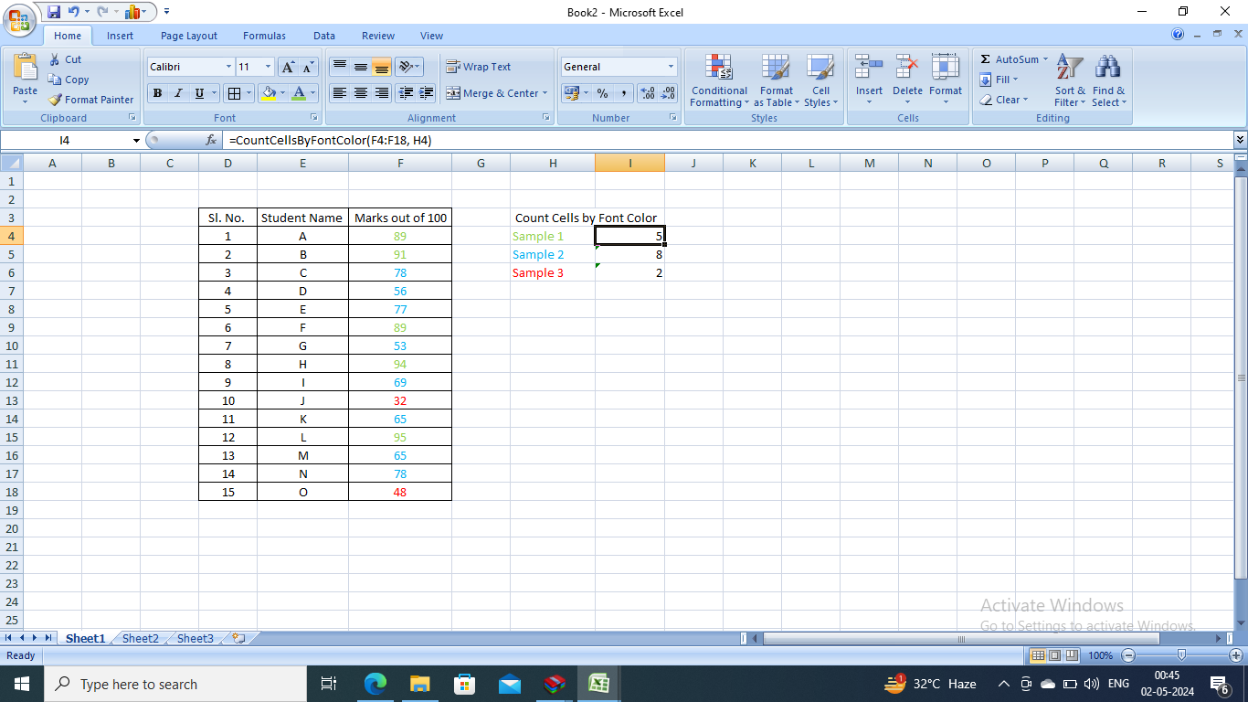
This way, the result will appear on your screen.

Finding the Sum by Cell Color in Excel

To find the sum, colored cells in Excel can be employed simply by using two formulae. I’ve discussed them below:

Sum in Excel by Cell Color

This function is not available on Excel by default; you will have to add it. To add the function, press “Alt+F11” and open the Microsoft Visual Basic window.

Go to “Insert” and click on “Module”. There, insert the code:

Function SumCellsByMatchingColor(targetRange As Range, referenceColor As Range) As Double
Dim colorToMatch As Long
Dim currentCell As Range
Dim totalSum As Double
' Set the volatile flag to ensure recalculation on changes
Application.Volatile
' Initialize the total sum
totalSum = 0
' Extract the color value from the reference cell
colorToMatch = referenceColor.Cells(1, 1).Interior.Color
' Loop through each cell in the target range
For Each currentCell In targetRange
' Check if the cell's interior color matches the reference color
If currentCell.Interior.Color = colorToMatch Then
' Add the cell's value to the total sum if there's a match
totalSum = totalSum + currentCell.Value
End If
Next currentCell
' Return the final sum as a double (to handle various data types)
SumCellsByMatchingColor = totalSum
End Function

This will add the function to your workbook.

Now, prepare your dataset.

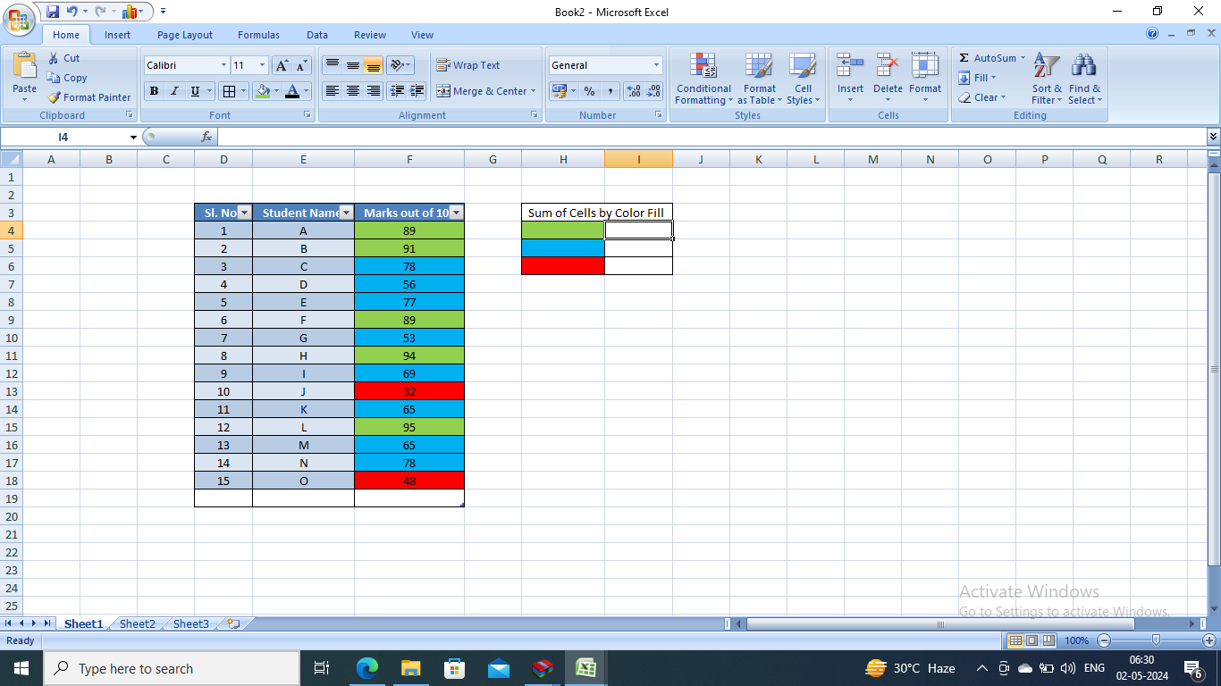
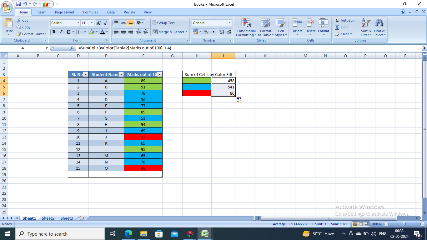
To find the sum of the values in cells that are colored green, use the formula

=SumCellsByColor(Table2[Marks out of 100], H4).

Once you obtain the result, drag and drop to the next two cells to get the sum of the values in blue and red cells as well.

Sum in Excel by Font Color

You will first have to add the function to your workbook. Follow a procedure similar to the one you used while adding the countcellsbycolor function.

Press “Alt+F11” to open the Microsoft Visual Basic.

There, use the code:

Function SumCellsByMatchingFontColor(targetRange As Range, referenceColor As Range) As Double
Dim referenceFontColor As Long
Dim currentCell As Range
Dim totalSum As Double
' Set the volatile flag to ensure recalculation on changes
Application.Volatile
' Initialize the total sum
totalSum = 0
' Extract the font color value from the reference cell
referenceFontColor = referenceColor.Cells(1, 1).Font.Color
' Loop through each cell in the target range
For Each currentCell In targetRange
' Check if the cell's font color matches the reference color
If currentCell.Font.Color = referenceFontColor Then
' Add the cell's value to the total sum if there's a match
totalSum = totalSum + currentCell.Value
End If
Next currentCell
' Return the final sum as a double (to handle various data types)
SumCellsByMatchingFontColor = totalSum
End Function

Now, you are ready to use this function in your workbook.

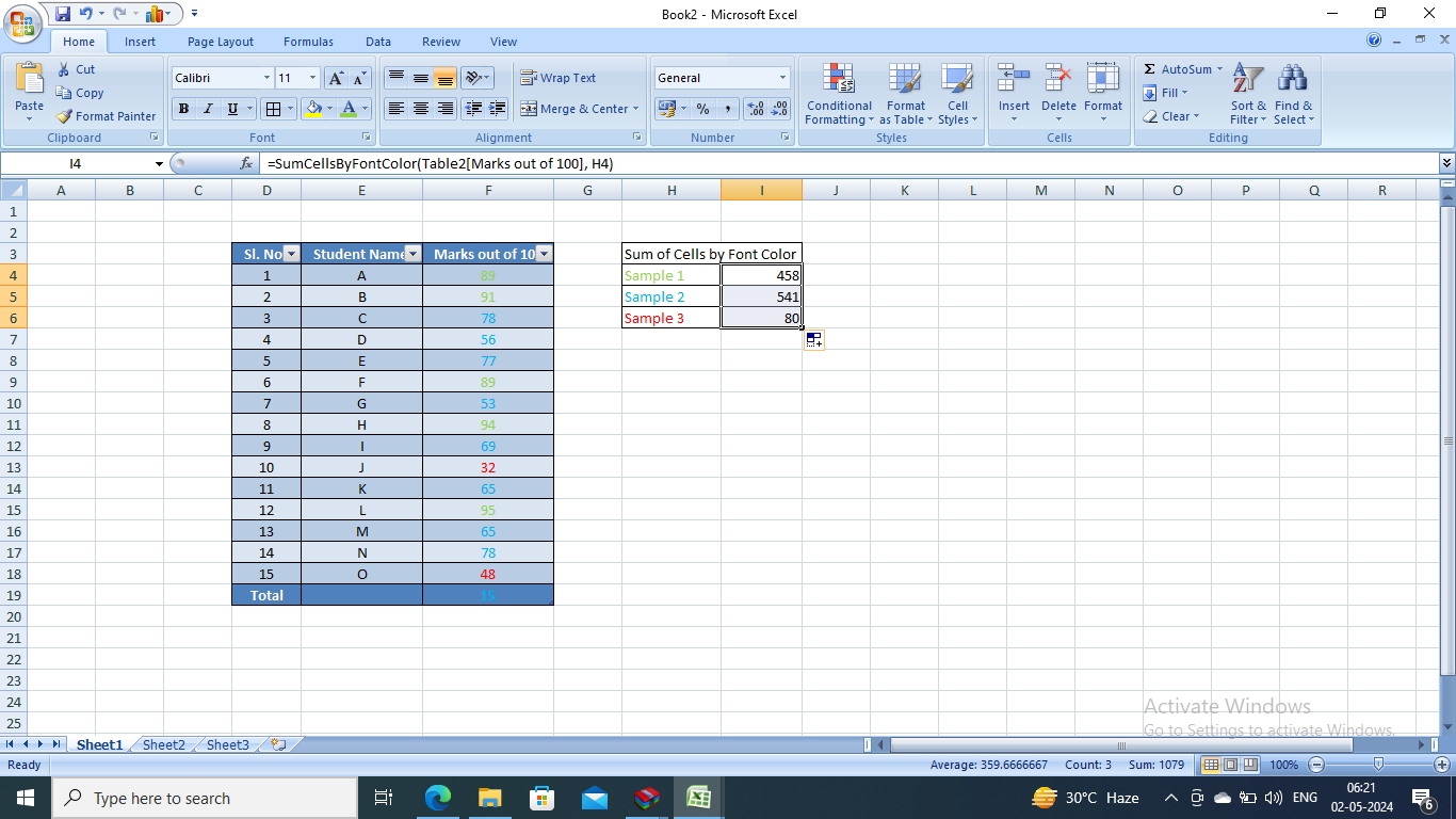
First, prepare your datasheet like this:

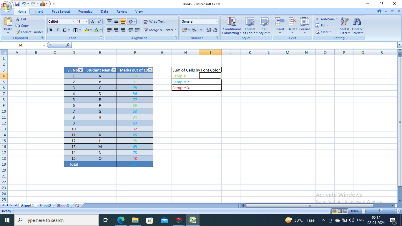
To find the sum of cells whose font is green, go to the cell where you want the result displayed and enter the formula =SumCellsByFontColor(Table2[Marks out of 100], H4). This will give the sum of all the values written in green.

Drag and drop in the next two cells to apply the same to them.

Count Colored Cells in Excel with the Help of a Table

If you are not very confident about adding a function in your workbook, you can still count colored cells in Excel. The steps I am mentioning below are an alternate way of counting colored cells without VBA.

• Step 1: Isolate the colored cells. This helps in saving time.
• Step 2: Select the entire table and press Ctrl+T to create a table. Since my dataset has headers, I will check the box that reads “My table has headers” and click on “OK.”

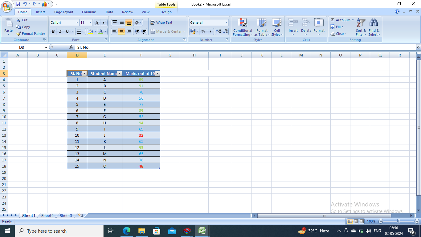
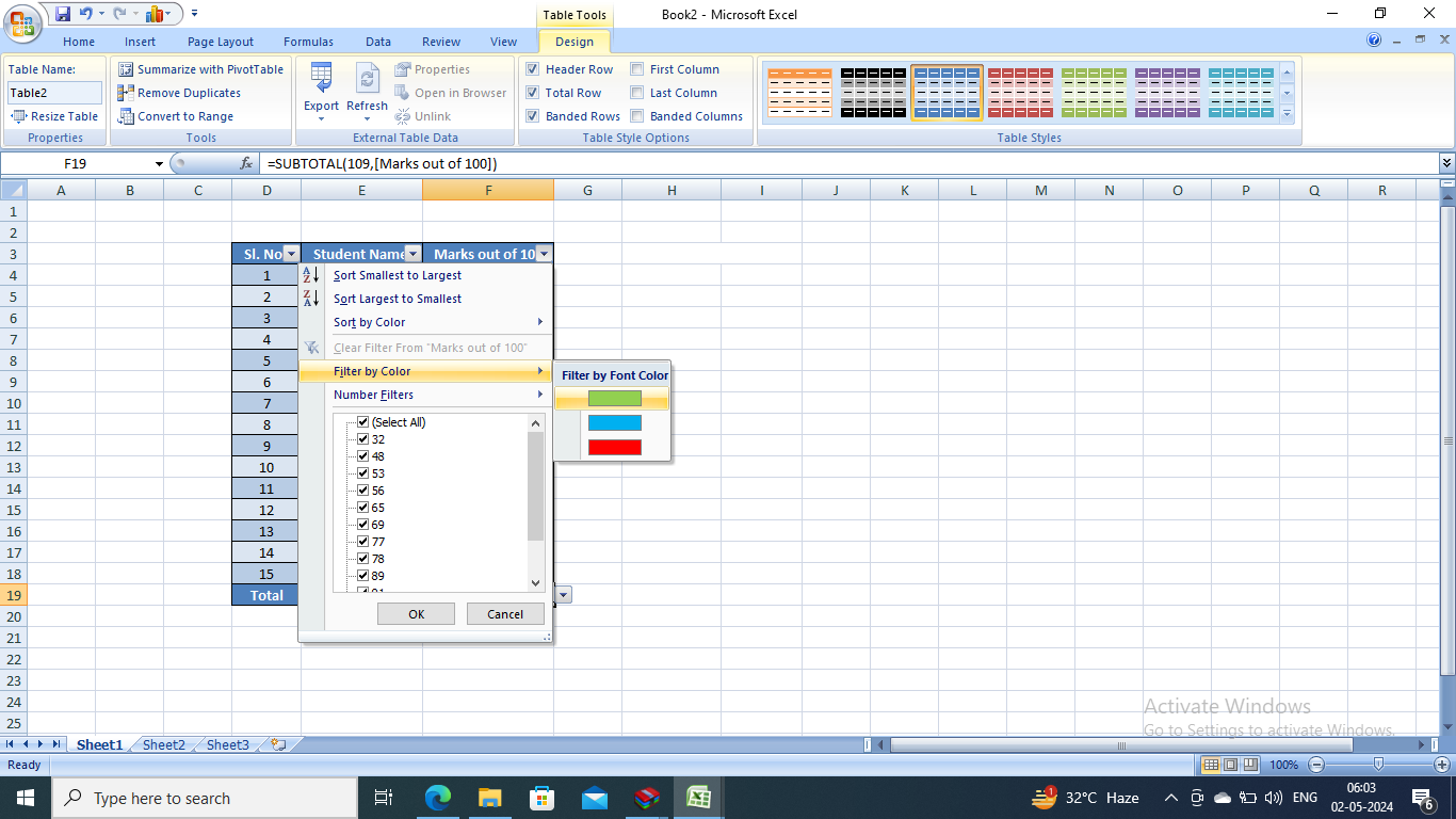
• Step 3: From the “Design” tab, go to the “Total row” option and check the box. A row will be added to the bottom of the table.

• Step 4: The “Total” row contains the sum total of all the data you have inserted. If you click on the cell that contains the “sum” value, you will see a drop-down menu of options.

If you want to count only the cells containing green font, first add the filter “Filter by Color” and choose the green color.

• Step 5: Next, click on the drop-down next to the cell containing the total value and click “Count.”

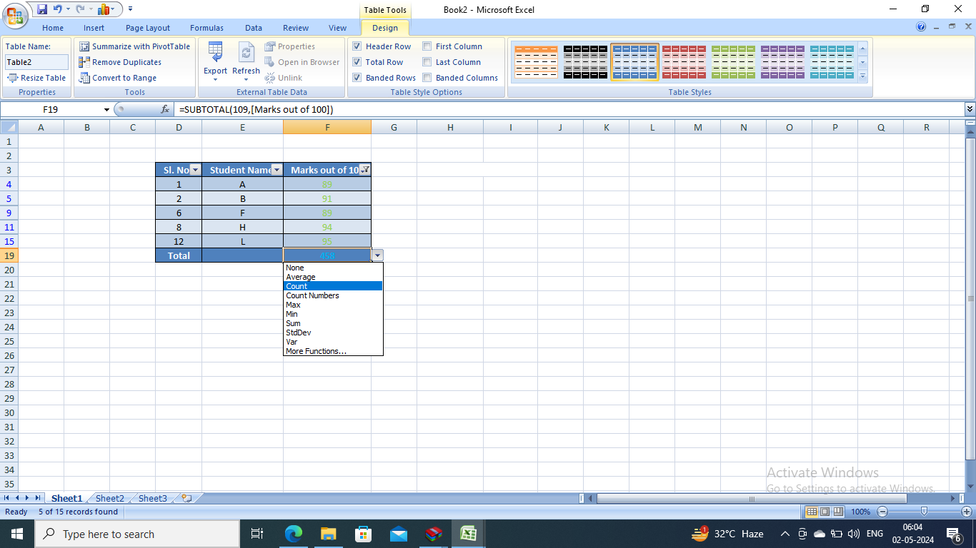
You will get the result. The cell will contain the value denoting the number of cells whose contents are written in green.

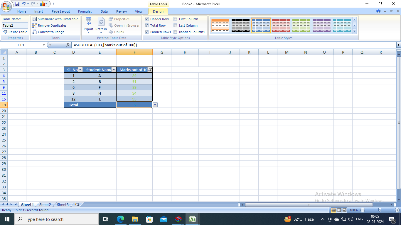
Count Colored Cells in Excel Using the SUBTOTAL Function

You can also count colored cells in Excel using the SUBTOTAL function. Have a look at the steps that I have mentioned below:

• Step 1: Prepare the data sheet and add filters. Go to “Sort and Filter” and click on “Filter”.

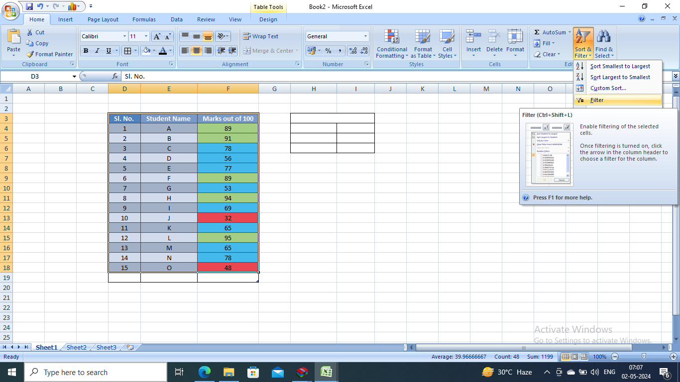
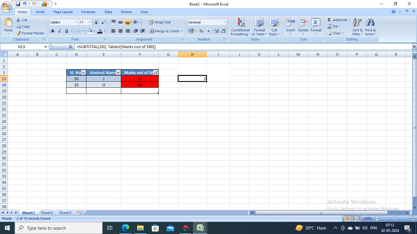
• Step 2: Now, in any cell where you want the result to be displayed, write the formula =SUBTOTAL(102, Table2[Marks out of 100]); where 102 denotes the count function in Excel, and the next argument denotes the cell range we are computing.
• Step 3: On pressing enter, you will get the total count. From the drop-down option in the heading bar, choose the color whose cell count you wish to see, and the result will be right in front of you!

Wrapping Up

Once you plunge into the pool of Excel, you will come across endless opportunities that can make your day-to-day computing and data analytics tasks easy. You may not find all the functions by default, but adding them is not a mammoth task that requires immense coding capabilities!

Therefore, start learning from the leading industry experts and validate your knowledge with a certificate with upGrad’s free online certification course in Excel. Visit upGrad to explore courses and choose the one that suits you the best.

FAQs

1. How do I count the sum of colored cells in Excel?

You can count the sum of colored cells in Excel using the syntax =SumCellsByColor(Cell Range, Criteria). However, you will first have to add this function using Microsoft Visual Basic.

2. How do I count colored cells in sheets?

You can count colored cells in Excel sheets using the SUBTOTAL function, with the help of a table, or using the CountCellsByColor function. The tutorial above provides a detailed step-by-step explanation of all three.

3. How do I count colored cells in Excel calendar?

You can use the COUNTIF function to count colored cells in the Excel calendar. All you need to do is specify the criteria as the cell color. First, use "Conditional Formatting" to assign colors to different cells. Then, use COUNTIF(range, "color") to count cells with a specific color.

4. How do I sum colored cells in Excel without VBA?

If your data set is not very large, find the sum of colored cells in Excel using the =SUM function, followed by selecting the cells of the specific color. You can also apply a filter and sort the cells of the desired cell color, copy and paste them into the adjacent cells, and apply the autosum function.

5. How do you count colored cells in Excel with text?

An easier way to count colored cells in Excel with text is by using the SUBTOTAL function. A detailed guide on how to do it is explained in the tutorial above.

6. How do I sum and count cells by color in sheets?

A complete guide on how to sum and count cells by color in sheets is explained in the tutorial above.