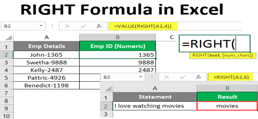
Excel RIGHT Function

Among the many functions that come handy while working on Excel, the RIGHT function deserves special mention. It reduces turnaround time for tasks, increases accuracy, and thus makes data segmentation easier. One formula that I find particularly useful is the Excel right function. This is a basic but multifaceted tool that retrieves a certain number of characters from the right side of a cell in your spreadsheet.

You can use the RIGHT function to deal with the data, such as customer IDs, product codes, filenames, or any other data that requires isolating the particular characters from the right end of a string.

This article delves into everything that you need to know about the RIGHT function in Excel, from its syntax and usage to the examples and the ways to solve problems that may occur while using it.

Source- EDUCBA

Mastering the Excel Right Function: Syntax, Usage, and Examples

Here's a breakdown of its syntax and usage:

Syntax: =RIGHT(text, num_chars)

Source- TrumpExcel

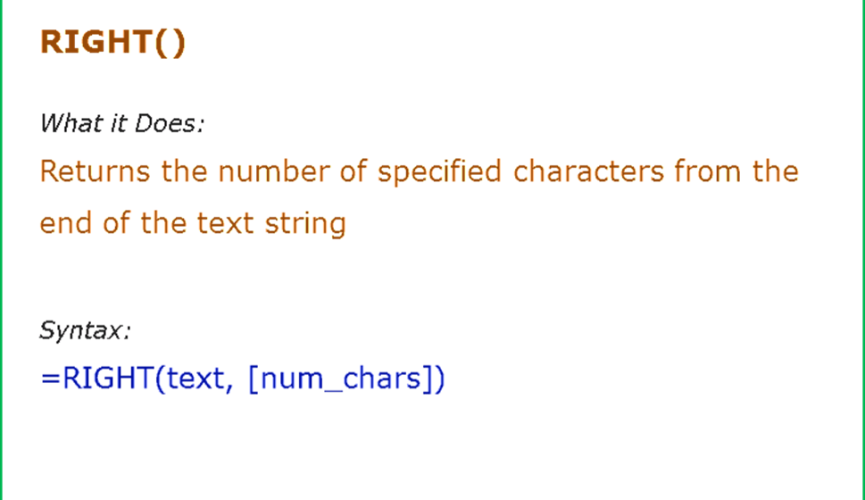
● text: This is the cell that has the cell reference containing the text string from which you want to extract the characters. Excel can process the text data that you paste directly into cells or the references to the cells that have text strings.

● num_chars: This is the number of characters you want to be taken from the right side of the text string. The aforementioned fact is that the num_chars should be a numeric value that is higher than zero. In case, you are going to key in a negative value for num_chars, Excel will respond with the #VALUE! error.

Example 1: Extracting the Last 3 Characters

Let's say you have a column of product codes in cell A1:A10. Every code has eight characters in it, and you, therefore, need to extract the last 3 characters (which may signify the product category).

Here's how you can use the Excel Formula Right

Excel =RIGHT(A1,3)

This Formula Excel Right shows how to take 3 characters (designated by the num_chars argument) from the right side of the text string in cell A1. In this situation, the formula will take the last 3 characters of the product code in cell A1 and show them in the cell where you have typed in the formula. You can then copy this formula down to the remaining cells in the column (A2:The work involved in A10) to get rid of the last 3 characters from all the product codes is certainly demanding. This can be even more handy when you have to sort or pick your data according to the specific ending codes.

Example 2: Extracting Everything After a Specific Character

Suppose you have a column of customer IDs in cell B1:B10, and each ID follows the format "CUS-#####". The aim is to get the unique ID number (the digits situated after the hyphen). Here's how you can combine the RIGHT function with FIND.

Here's an Excel Right Function Example with FIND:

Excel

=RIGHT(B1,LEN(B1)-FIND("-",B1))

This formula leverages the combined power of two Excel functions: Excel Right Function and FIND. The FIND function locates the position of the hyphen (-) within the customer ID text string in cell B1. Then, the LEN function determines the total length of the text string in cell B1. By subtracting the position of the hyphen (found by FIND) from the total length (found by LEN), we essentially calculate the number of characters to extract from the right side of the text string. Finally, the RIGHT function takes over, extracting that calculated number of characters from the right side of the text string in cell B1, effectively giving you the unique ID number.

This Excel Right Function after-character approach is useful when your data follows a consistent pattern with a specific separator character, allowing you to isolate the desired information. Moreover, you can refer to this Excel tutorial for guidance.

Wrapping Up

The Excel Right Function is a strong and user-friendly tool that you can easily add to your Excel list. By getting to know its syntax, applications, and how to use it in combination with other functions, you can efficiently process text data in your spreadsheets, thus, you will be able to save time and effort as well. Thus, whenever you need to get the exact characters from the right side of your text strings, the Right Function will be your friend and your Excel productivity will be at its peak.

If you want to improve your Excel skills and realize its full potential, you should take UpGrad courses on Excel which are comprehensive and cover the entirety of Excel. UpGrad has a variety of beginner to advanced programs that are designed to enable you to master the basic formulas, functions, and techniques. Through proper study methods, industry-based curriculum, and expert teachers, you can develop the confidence to face any Excel challenge and turn into a spreadsheet expert!

Frequently Asked Questions

1. How do you use the Excel RIGHT function in Excel?

The RIGHT function follows a specific formula syntax: =RIGHT(text, num_chars)In this situation, "text" denotes the cell where the text string you wish to extract the characters from is, and "num_chars" is the number of characters you want to extract from the right side. Refer to these Excel tips and tricks for more information.

2. How do I extract text from the right in Excel?

The Excel RIGHT function is your companion in the world of Excel when you want to get the text from the right part of a cell. Just copy the formula as it is and put the formula in the specified cell and the number of characters to be extracted.

3. What is LEFT () and RIGHT () in Excel?

Excel offers two counterpart functions: Leftward and rightward. The LEFT function functions to get the characters from the start of a text string, and the RIGHT function, as we're talking about, to get the characters from the end. These functions are the basic tools for working with text data in spreadsheets and are applicable in many situations.

4. How do I get everything right of a character in Excel?

You can obtain all the characters to the right of a specific character by combining the Excel RIGHT function with the FIND function. The FIND function identifies the location of the target character in the string of text, and it will then take everything from that point onwards. This is a flexible technique of extracting texts that follow a certain delimiter or separator in your data set.

5. What is the shortcut for RIGHT Function in Excel?

The RIGHT function does not have a unique keyboard shortcut. Nevertheless, you can use the Excel Formula Right in Formula Builder tool in Excel to build a custom shortcut that will be perfect for your work process. Here's how to do it:

Begin your performance by copying the Excel RIGHT Function in your spreadsheet cell (=RIGHT(text,num_chars)).

After you have formed the formula, press F2 to make changes to the formula in the cell directly.

Draw attention to the whole formula, after which you can right-click and choose the option "Assign Macro. . . " from the context menu.

In the "Assign Macro" dialog box, name your custom shortcut a memorable one (e. g. Quick Note, Fast Sigh). g. "ExtractRight") and click "OK".

Thus, when you need to use the Right function, just click Alt and the letter of your macro (e) at the same time. g., Alt+R for "ExtractRight"). This can be of great help because it can save you time in doing the right thing.

6. What is the RIGHT and Len formula?

The LEN function provides the length of the text string in an Excel spreadsheet. You can merge the Excel Right Function with LEN to obtain the specific number of characters from the end. To be more specific, to get the last 3 characters of a text string, you can use the formula =RIGHT(text, LEN(text)-3). This is a formula that finds out the total length of the text string using LEN and then subtracts 3 to find out the number of characters to be taken from the right side using RIGHT.