Excel Transpose Formula

While working with data in Microsoft Excel, the orientation in which the data is organized in cells plays quite an important role. Sometimes, you may have to rotate or switch the cells. 

But how do we go about it? Do we have to manually re-enter all the values? That is practically not possible for large data sheets!

I discovered that the Excel Transpose option is the perfect solution to this. 

The Excel Transpose option helps users easily switch between rows and columns as per their requirements. This simplifies tasks like manipulation of data, helps in easier analysis, and allows great presentation of information, thereby making the data management process more flexible. 

In this tutorial, I will discuss the different ways in which you can use the Excel Transpose function. Read on. 

What is Transpose in Excel?

Let us start with the basic understanding of Excel Transpose. 

Do you want to change the orientation of data in your Excel sheet? You will have to use the Excel Transpose function. This way, you will be able to convert a horizontal range to a vertical range, and vice versa. 

Rearranging a dataset makes it easier to analyze data, or offers better readability. This is especially helpful in creating summaries and reports, as it presents data in a meaningful and more organized manner. 

After reading this tutorial, you will be able to apply the Transpose function (Excel) in three different ways: 

• By using the Paste Special Transpose option
• The built-in Transpose function
• The Power Query tool 

When transposing data in Excel, functions like TRANSPOSE offer a convenient way to restructure information. They are powerful tools for data manipulation and analysis. They enable users to perform various tasks efficiently, such as calculations, formatting, and data organization. 

To deepen your understanding of Excel functions and enhance your skills, consider exploring comprehensive tutorials or courses on Excel functions.

Paste Special Transpose

With the help of Paste Special Excel Transpose, we can easily control the formatting of the content that we are pasting. I am listing down the steps below:

• 1st step: You will first have to select the range that you wish to transpose. 

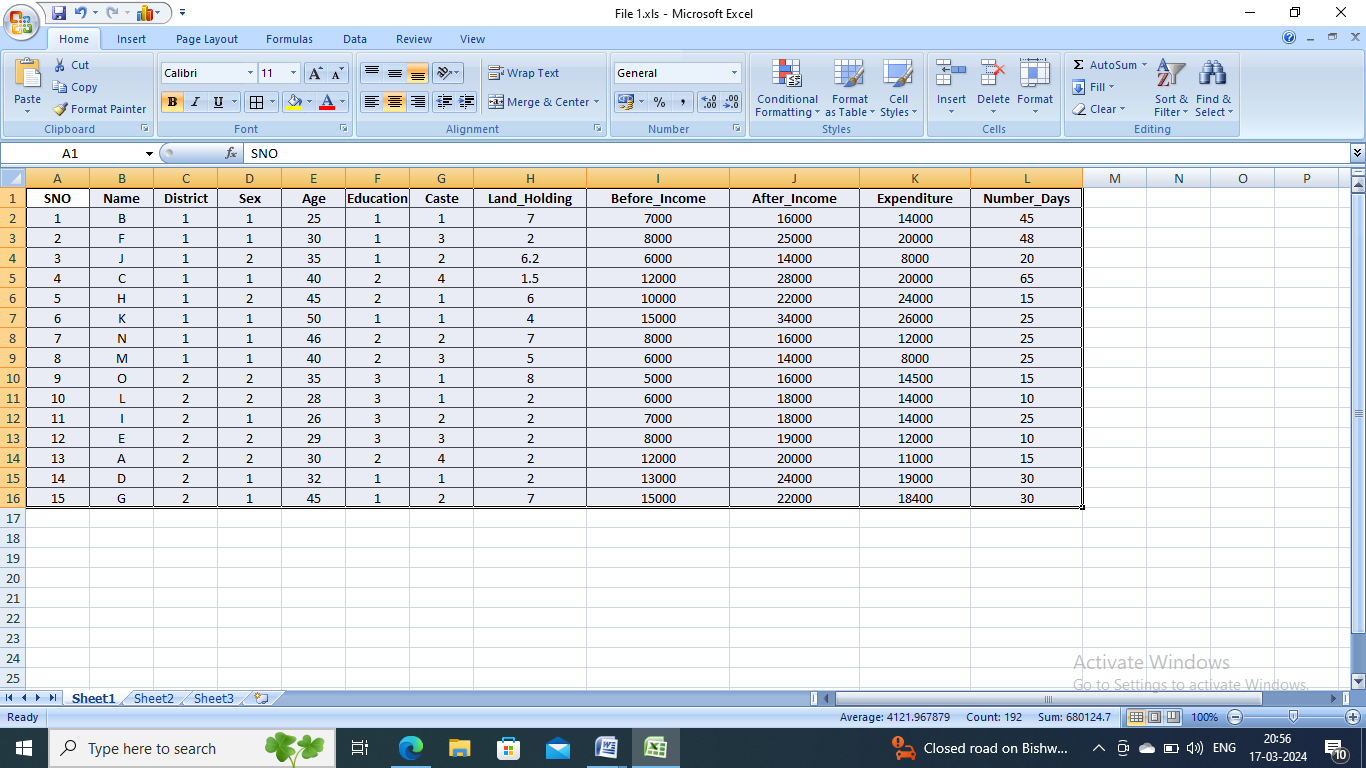
Source: MS Excel

• 2nd Step: Next, go to the Home tab and choose the “Copy” option. You can also right-click on the entire range and choose the Copy option. 

• 3rd Step: After you have copied the data, choose the destination where you want the transposed data to be pasted. 
• 4th Step: Go to the Home tab, choose the Clipboard section, next go to Paste, and finally click on Paste Special. You can also accomplish this task more efficiently. You will have to right-click on the cell where you want the transposed cells to be pasted. 

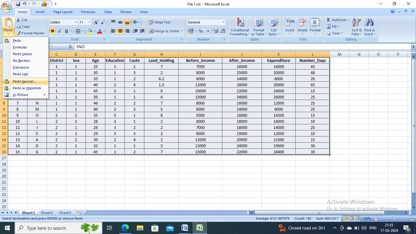
Source: MS Excel

• 5th Step: Once the Paste Special dialogue box appears, click on “Values” and choose the “Transpose” option that is present on the bottom right. 
• 6th Step: Click on OK and the result will appear on the screen. The data set will be transposed to your new desired location. 

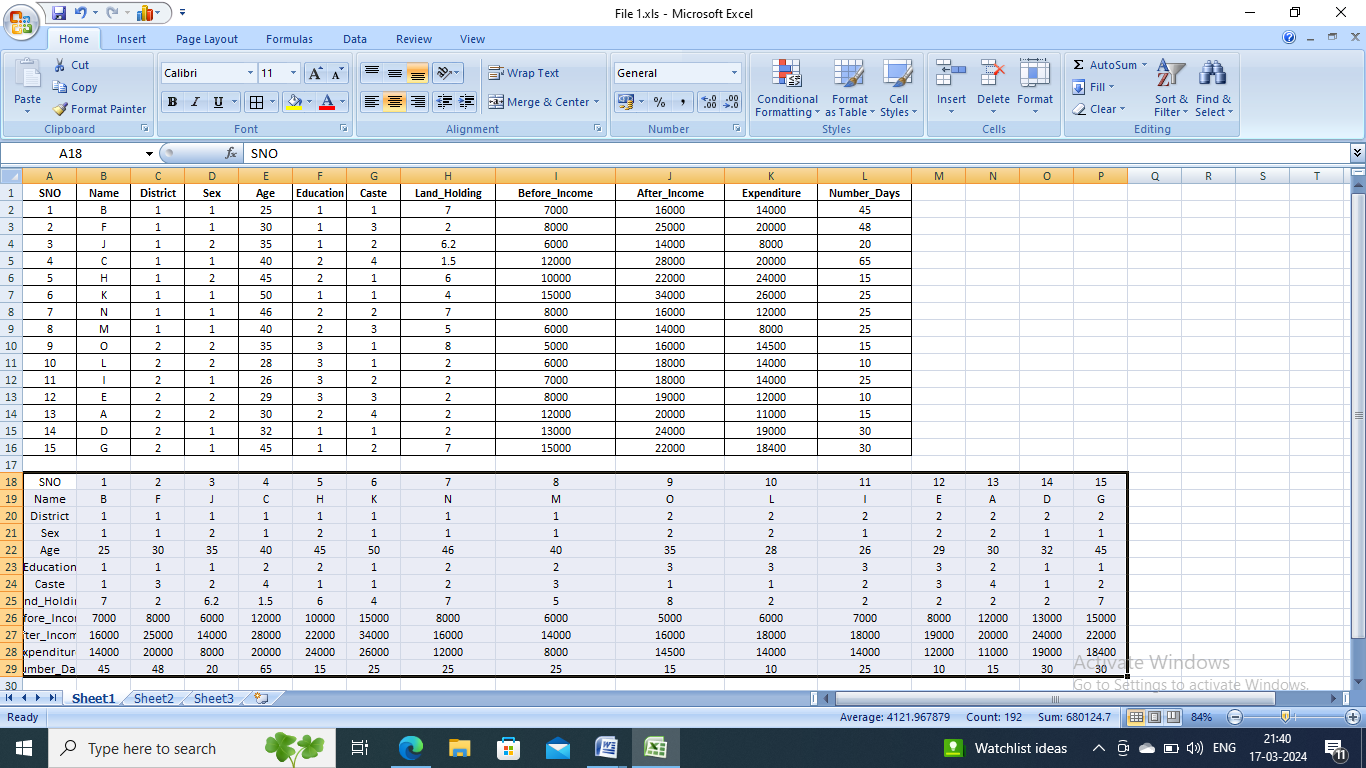
Source: MS Excel

Hope this gives you an idea about the technique of data transpose in Excel using the Paste Special option. Let us now move to understanding how to use the in-built “Transpose” function in Excel. 

In-Built Excel Transpose Function

Excel has an in-built Transpose function that can be used to transpose data in Excel. The syntax to be used for this function is =TRANSPOSE(array). Here, “array” refers to the range of cells that you wish to transpose. 

The steps you need to follow to use this Excel Transpose function are:

• 1st Step: You will first have to select the cell range where you want to transpose the data set. 
• 2nd Step: If the range of your table is 5x6, i.e. 5 rows and 6 columns, you will have to select 6 rows and 5 columns where you wish the output transposed data to appear. 

Source: MS Excel

• 3rd Step: Next, you will have to enter the formula =TRANSPOSE(A1:F5). 
• 4th Step: It is important to note that you should not press “Enter” to execute array formulas. Instead, you will have to press Ctrl+Shift+Enter. This helps to put braces around the formula. This helps to impart the message that the output will not be a single cell, but an array of data. 
• 5th Step: After this, your data will be transposed. 
  

Transposing Tables Without Zeros

While working, I also found that the Excel Transpose function converts the blank cells into zero. Don't worry; I’ve got the solution for this too!

To copy blank cells as they are while transposing, you need to use the IF function with TRANSPOSE. 

The formula for this is =TRANSPOSE(IF(A1:F5=””,””,A1:F5)). The IF function helps to look for blank values and return them as empty strings at the time of transposing. 

Power Query Tool for Transposing Data

This is one of the most powerful built-in data automation tools that is available in Microsoft Excel. 

Using this tool, you can easily transpose your dataset. The steps you need to follow are mentioned below:

• Select the data range: Highlight the cells containing the data you wish to transpose.
• Go to the Data tab: Navigate to the "Data" tab in the Excel ribbon at the top of the window.
• Access "Get & Transform Data": Under the "Get & Transform Data" section, click on the option labeled "From Table/Range".
• Open Power Query Editor: This action will open the Power Query Editor, displaying your data.
• Navigate to the Transform tab: Within the Power Query Editor, switch to the "Transform" tab located in the ribbon.
• Adjust Headers: In the "Table" section, locate the option to set headers as the first row. Click on it to ensure that all headers are moved to the first row.
• Transpose the data: Once the headers are correctly positioned, locate and click on the "Transpose" option.
• Close and Load: After transposing the data, click on the "File" tab, and select "Close & Load" to exit the Power Query Editor and load the transposed data into your Excel worksheet.

The result will appear on the screen. You will see that the transposed data will be loaded into a new Excel sheet. 

Having a good command over data management can prove to be beneficial in the long run. You can opt for an Excel or any other data science and analytics course to learn more about these concepts. 

Summing Up

Hope this gives you an overall idea about how to transpose row to column in Excel in three different ways. This will help to save a lot of time that would be otherwise spent in entering the data manually. 

There are endless functions in Excel that can help you perform your tasks efficiently and save time. From basic arithmetic operations to complex data analysis, Excel offers a vast array of functions to streamline your workflow. The more time you spend using Excel, the more you will be able to discover the hacks that will save you time and make your tasks easier. Consider delving into tutorials or courses on Excel functions to unlock its full potential.

upGrad offers a wide range of courses specially designed for working professionals who are looking forward to upskilling themselves. All the course curriculums are designed by industry experts. Learners also get advantages like flexible payment options and lucrative job opportunities. 

Frequently Asked Questions

1. How do you transpose data in Excel?

There are three ways in which you can transpose data in Excel; the Paste Special Option, the Built-in Transpose Function, and the Power Query Tool 

2. How do I flip data vertically in Excel?

To flip data vertically or horizontally, you will have to transpose your data in either of the three ways mentioned above. 

3. How do I change data from columns to rows in Excel?

The Excel Transpose option helps to change data from columns to rows in Excel.

4. What is the shortcut for Transpose in Excel?

The Excel Transpose shortcut for transposing cells including the formatting is Ctrl+Alt+V and then E. If you want to transpose only the values, use Ctrl+Alt+V and then E, V, and Enter. 

5. What is a Transpose formula?

The formula for Transpose is =TRANSPOSE(cell 1:cell 2).

6. Is there a formula to Transpose?

Yes, in Excel, the TRANSPOSE function can be used to transpose a range of cells or an array. It converts rows into columns and vice versa. For example, if you have data in cells A1:B3 and you want to transpose it to cells D1:E2, you can use the formula =TRANSPOSE(A1:B3) entered as an array formula by pressing Ctrl+Shift+Enter.