H LOOK UP in Excel

Once, I had to work on a last-minute assignment on summarizing sales. I was pretty sure that I wouldn’t make it on time but luck had something else for me.

I immediately recalled the spreadsheet trick from the old days. Besides, the sales report had all the necessary codes in the first column, and the remainder of the figures in the next ones. Perfect for an H LOOK UP in Excel (Correct format: HLOOKUP)!

Aside from the numerous other Excel functions I was well-versed in, knowing this one surely saved the day. Starting from sorting data to saving data in my projects, this function has helped me a great deal till this day.

If you wish to learn how I did, keep reading about how an Excel HLOOKUP function can benefit you too!

What is H LOOK UP in Excel?

The HLOOKUP function in Excel stands for horizontal lookup. This function helps you identify a specific value in a row, also known as a table array. By executing this function, you can find the same value from a different row in the same column.

Syntax

Let's understand the syntax of the H LOOK UP formula in Excel:

HLOOKUP(lookup_value, table_array, row_index_num, [range_lookup])

• Lookup value (required): What you're searching for (e.g., product name)

• Table array (required): The range of cells containing your data table. This is also a required category.

• Row index number (required): The specific row you want to retrieve information from (starting from 1).

• Range lookup (optional): How strict you want the search to be

• TRUE (or null): This finds the closest value less than or equal to what you're searching for (in an approximate match). You can opt for this if your data isn’t perfectly sorted to begin with.

• FALSE: This only returns an exact match, otherwise returns an error (#N/A.) I’d recommend using this if your data lies in ascending order.

Example of HLOOKUP Function

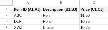
Imagine a data table with product codes placed in the first row.

Let’s call it A1:D1 and add the corresponding prices in the second row (A2:D2). Your goal is to find the price of the product with the code “ABC which is located in cell B1.

Here’s how you should put your values for the ideal results.

According to the HLOOKUP in Excel formula, your syntax should look like this:

=HLOOKUP("ABC", A1:D1, 2, FALSE)

To break down your syntax, this is the explanation:

• The code we’re searching for is ABC (lookup_value).
• The data table exists in the range A1:D1 depicted by (table_array).
• The second row tells you the price (row_index_num = 2) as the first one contains the codes.
• Since the codes are likely to be unique, we’re looking at an exact match with (range_lookup = FALSE).
  

Additional remarks

• Sort the first row of your data table for efficient searching with TRUE in range_lookup.
• Incorrect row numbers or missing values will result in errors (#VALUE! or #REF!).
  

How to use the HLOOKUP in Excel with Formula

A prerequisite to using H LOOK UP in Excel is to find the purpose of the function. By now, you’d have guessed that we are trying to explore a value in a horizontally-arranged table. Let’s start the next steps now:

Step 1. Identify your data

Locate the data table that you’re going to work with and ensure the lookup value exists in the first row of the table.

Step 2. Set up the HLOOKUP formula in Excel with example

Click on the cell in which you want the result to be displayed. After that, type HLOOKUP(.

Step 3. Enter the arguments

• Lookup value: Inside the first bracket, specify the value you're searching for. This can be a direct value, a cell reference, or a formula that evaluates the search value.

• Table array: Separate the lookup value with a comma (,). Then, enter the range of cells that includes your entire data table. You can either type the cell range (e.g., A1:D10) or select the table area with your mouse.

• Row index number: Separate the table array with a comma (,). Enter the number indicating the row from which you want to retrieve data after finding the match in the first row.

Think of it as moving down vertically. A value of 1 retrieves from the second row (excluding the first row which holds your lookup criteria), 2 retrieves from the third row, and so on.

• Range lookup (optional): Add another comma (,). This argument determines how strict the search should be.

• TRUE (or omitted): This enables an approximate match. If the exact value isn't found in the first row, HLOOKUP returns the closest value less than or equal to your search term. This is useful when your data isn't perfectly sorted.

• FALSE: It enforces an exact match. If no perfect match exists in the first row, HLOOKUP returns an error (#N/A).

Step 4. Complete your formula

Finally, close the parentheses after your last argument, thereby completing the formula. Following that, press Enter and Excel will evaluate the formula for you.

Conducting an Approximate Match in HLOOKUP: Step By Step

Here's how to conduct an approximate match using HLOOKUP in Excel:

Step 1. Set up your data

Ensure your data is in a table format with the lookup values in the first row.

Step 2. Build the formula and press Enter

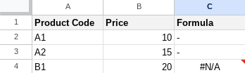
In the desired cell, type =HLOOKUP("XYZ", A1:D3, 3, TRUE)

Imagine this table (A1:D3):

Result: This formula will return $0.75, the price of the closest item (DEF) because "XYZ" is not present.

Conducting an Exact Match in HLOOKUP: Step By Step

Here's how to conduct an exact match in HLOOKUP with an Excel table:

Steps:

Step 1. Prepare your data

Organize your data in a table format and ensure the lookup value you want to find is present in the first row of the table.

Step 2. Set up the formula

Click on the cell where you want the result to be displayed and type `=HLOOKUP(`

Step 3. Enter the arguments and complete the formula

Write the formula and type the cell range (e.g., A1:D10) or select the table area.

Source - MS Excel

Imagine you have a data table in cells A1:D2 with product codes (A1:A2) and corresponding prices (B1:B2). You want to find the exact price of the product with code "ABC" (located in B1).

Syntax: =HLOOKUP("ABC", A1:D2, 2, FALSE)

VLOOKUP and HLOOKUP: Difference

Understanding the difference between the two functions is as easy as understanding directions to a street.

The VLOOKUP function essentially deals with vertical lookups and retrieves data from the same column in a different row. Hlookup does just the opposite by retrieving data from the same column but different rows. Here’s a table:

To conclude, VLOOKUP is more sought after within Excel as it can gather wider info from a wider range of applications.

How to Extract HLOOKUP in Excel From Another Worksheet or Workbook

Example: You have data in Sheet 2 (A1:D10) of the current workbook and want to find the price of a product with code "ABC" (located in cell B1 of this sheet).

For Worksheet

Formula (assuming data is in Sheet 2):

=HLOOKUP("ABC", 'Sheet2'!A1:D10, 2, FALSE)

For Workbook

Assuming that the data exists in a different workbook named “data.xls

=HLOOKUP("ABC", [C:\Users\Documents\data.xlsx]Sheet1!A1:D10, 2, FALSE)

How to Use HLOOKUP in Excel to Return Multiple Values

There are two ways to go about it.

1. Using an Array formula

By using this method, you can manipulate the formula to return an array of your desired value.

Syntax: {=HLOOKUP(lookup_value, table_array, ROW(A1:A1)+row_index_offset-1, FALSE)}

2. Using INDEX and MATCH

I prefer this method more as it gives me the liberty to trace multiple values.

Syntax: {=INDEX(table_array, MATCH(lookup_value, first_column, 0), column_index_offset+COLUMN(A1)-1)}

Common HLOOKUP Problems and Their Solutions

Is your HLOOKUP not working? Here’s what you need to do to eliminate all discrepancies:

• Incorrect formula in syntax: Double-check for typos, missing parentheses, or misplaced commas. Ensure the formula structure follows:

=HLOOKUP(lookup_value, table_array, row_index_number, [range_lookup]).

• Mismatch in data type: Inconsistent data types between the lookup value and the first row of the table can lead to errors. Use functions like TEXT or VALUE to ensure they match.

• Missing lookup value: The value you're searching for might not be present in the first row, resulting in an error. Verify its existence.

• Incorrect row index number: Entering a value less than 1 or exceeding the number of rows will cause issues. Ensure the row index aligns with your desired data location.

• Unsorted data and approximate match: If your data isn't sorted in ascending order and you're using approximate match (TRUE), HLOOKUP might return unexpected results. Sort the data or switch to an exact match (FALSE).

Although this is a quick an easy guide, to gain in-depth knowledge about this software, do consider taking up professional Excel certification courses to hone your skills.

Wind up

The function, H LOOK UP in Excel is by far one of the most versatile Excel functions I’ve used to date. Having said that, I think you should give it a try and see for yourselves.

So far, I have established the usability of HLOOKUP in Excel determining the expected results. But did you know that you could go ahead and excel at Excel too? With upGrad’s array of courses, you can avail the top certifications and get working in no time.

Learn now!

Frequently Answered Questions

1. What is lookup in Excel?

Lookup is an Excel function that allows you to search for something specific within your spreadsheet. H LOOK UP in Excel is designed particularly for a horizontal lookup.

2. How is VLOOKUP used in Excel?

You can use the VLOOKUP function by searching for a specific value in one column and retrieving data from a different one.

3. What is HLOOKUP vs VLOOKUP?

The difference between VLOOKUP and H LOOK UP in Excel is an easy one. You use HLOOKUP when looking to extract data from a horizontal lineup whereas VLOOKUP works in the vertical front.

4. How to do a lookup field in Excel?

You can exercise the lookup function based on your data structure. You can either use the function manually or look it up using the Lookup Wizard. To do it manually, use this reference:

VLOOKUP(lookup_value, table_array, col_index_num, [is_sorted]).

5. What is the lookup formula?

When it comes to a formula HLOOKUP is used to retrieve data using specific values. Several lookups exist, however, the big shots are HLOOKUP (horizontal lookup) and VLOOKUP (vertical lookup.)

6. What is a Lookup table with an example?

A lookup table is a reference table used to retrieve information based on a key or identifier. For instance, in a customer database, a lookup table might match customer IDs with their corresponding names and contact details, facilitating quick access to specific customer information.

7. What is Hlookup vs VLOOKUP?

The main difference between VLOOKUP and H LOOK UP in Excel is that HLOOKUP searches for the value in the first row of a table (horizontal lookup), while VLOOKUP searches for the value in the first column of a table (vertical lookup).

8. How to do a lookup field in Excel?

To make a lookup field in Excel, use VLOOKUP. Input "=VLOOKUP(lookup_value, table_array, col_index_num, [range_lookup])", substituting terms accordingly.