How To Freeze Panes in Excel

When you’ve got plenty of data at your disposal, it may get difficult to distinguish items in your notebook. Fortunately, Excel offers an abundance of functions and capabilities that make it easier to look over information from many sections of your notebook at the same time.

With experience of more than a decade as a techie, I have understood how to freeze panes in Excel. Excel online courses sure helped me get started with honing my skills in this software. It has also helped me try out new functions and methods to manage my worksheet and easily freeze panes. Hence, in this tutorial, I’ll help you understand the same.

How to Freeze the Top Row in Excel?

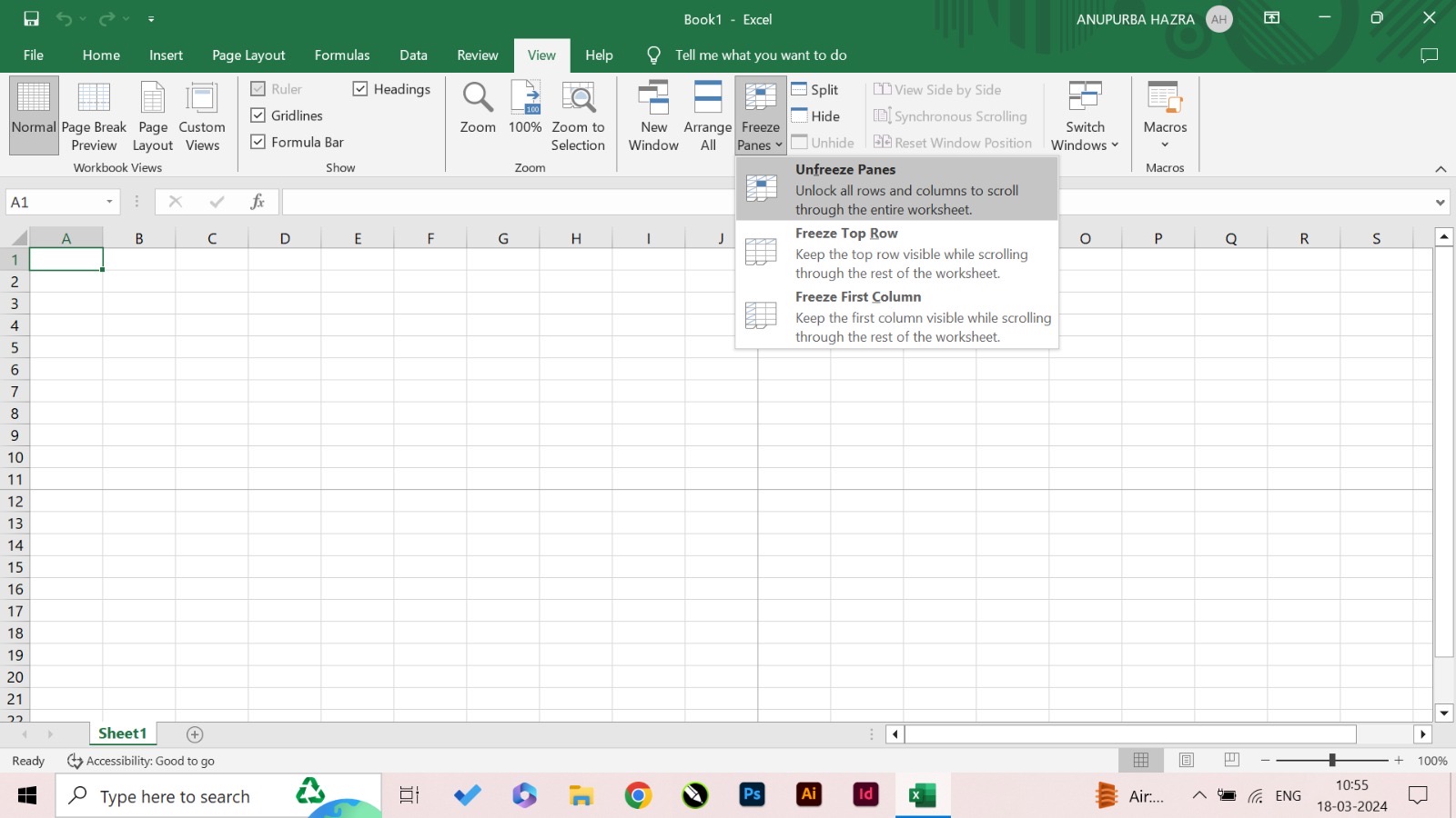
Let me illustrate how to freeze rows and columns in Excel so that you can conveniently manage large amounts of data contained in a table. Follow the below-mentioned steps to successfully freeze the Top row in Excel:

1. Select the option of ‘freeze panes’ in the view tab that is displayed on the Windows bar.

2. Click on ‘freeze top row’ and scroll down to make use of the rest of the worksheet.

3. You will automatically notice a dark gray horizontal line covering the top row, which shows that the top row is frozen.

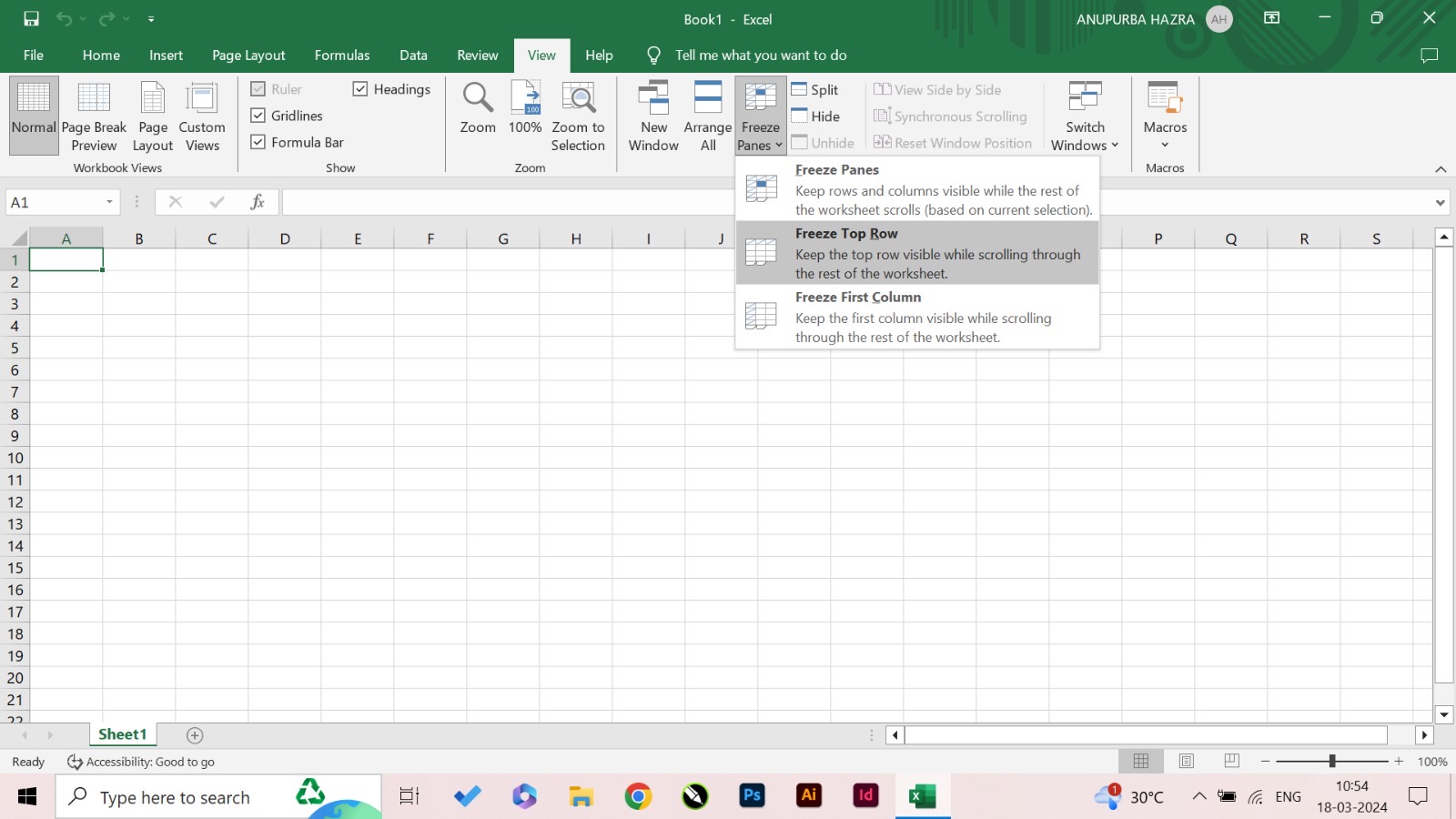
Source: MS Excel

Following this, you’ll be able to freeze the very first row in the Excel spreadsheet

How To Freeze Multiple Rows in Excel?

As a beginner in the tech industry, I always wondered how to fix row in Excel without creating much hassle through the worksheet. While nifty Excel functions simplify calculations, there are also straightforward methods to lock multiple rows.

In certain scenarios, you may want to freeze more than one row, and doing it one by one can be very time-consuming. Learn how to freeze panes in Excel in case of multiple rows by following these steps:

Source: MS Excel

1. Select the row that is just below the concluding row that you want to freeze or simply choose the row’s first cell.

2. Then move to the view tab and opt for ‘freeze panes’ and you’re done. Now you know how to freeze selected rows in Excel.

How To Freeze the First Column in Excel?

In my years of experience, this is the easiest way in which I learned how to fix a column in Excel and trust me, you can do it at your fingertips. Here’s how to freeze columns in Excel:

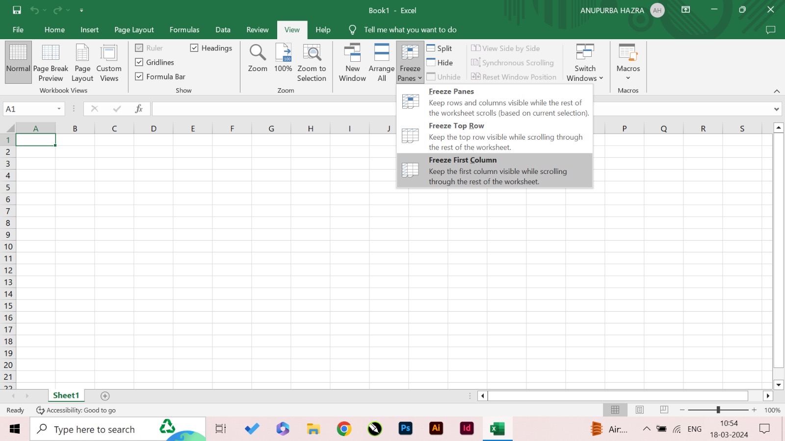
Source: MS Excel

1. Select ‘freeze panes’ from the view tab in the Windows section.

2. Opt for ‘freeze first column’ from the toolset.

3. Move to the top-right corner of the spreadsheet to freeze panes in Excel.

How To Freeze Multiple Columns in Excel?

Selecting and freezing one column at a time can be very tiring. So to make it simple and quick, you can lock numerous columns at once. Follow the below-mentioned steps to learn how to freeze multiple columns in Excel.

Source: MS Excel

1. Select the column that is right to the final column that you want to freeze or simply choose the column’s first cell.

2. Then move to the view tab and choose the option of ‘freeze panes’ and you have it.

The spreadsheet will automatically show dark gray lines on the columns that you have locked. Keeping them aside, you can navigate across the rest of the worksheet. Usually, beginners get perplexed when they are asked how to freeze bases in Excel but in reality, it is not a difficult task at all.

How to Freeze Cells in Excel?

When you want to lock rows and columns together, it means you are indicating a cell. It becomes easier for you to lock a cell with one single function, rather than freezing rows and columns, individually. To learn how to freeze rows and columns in Excel, follow the below-mentioned steps:

1. Firstly, choose a cell that you want to freeze which is just above the last row and just right to the final column.

2. Click on the View tab and opt for ‘freeze panes’ and you are done.

Source: MS Excel

A dark gray box will automatically appear in the intended cell which indicates that the particular cell is locked. You can move through the rest of the spreadsheet just as you like.

What is the Magic Freeze Button in Excel?

Here’s another interesting way to learn how to freeze panes in Excel; the magic freeze button. What is it and how does it work? Let’s understand in detail.

You can instantly freeze the first row or the first column multiple rows and multiple columns or an entire cell by employing the magic freeze button. You can conveniently add the magic free button from the quick access toolbar.

1. Click on the arrow on the quick access, toolbar and opt for ‘more commands’.

2. Select the option of ‘commands not in the ribbon’ from the ‘choose command’ section.

3. Click on ‘freeze panes’ and then ‘add’.

4. Click on the ‘OK’ button.

5. If you wish to freeze the Top row, then select the entire row and opt for the magic freeze button and it’s done.

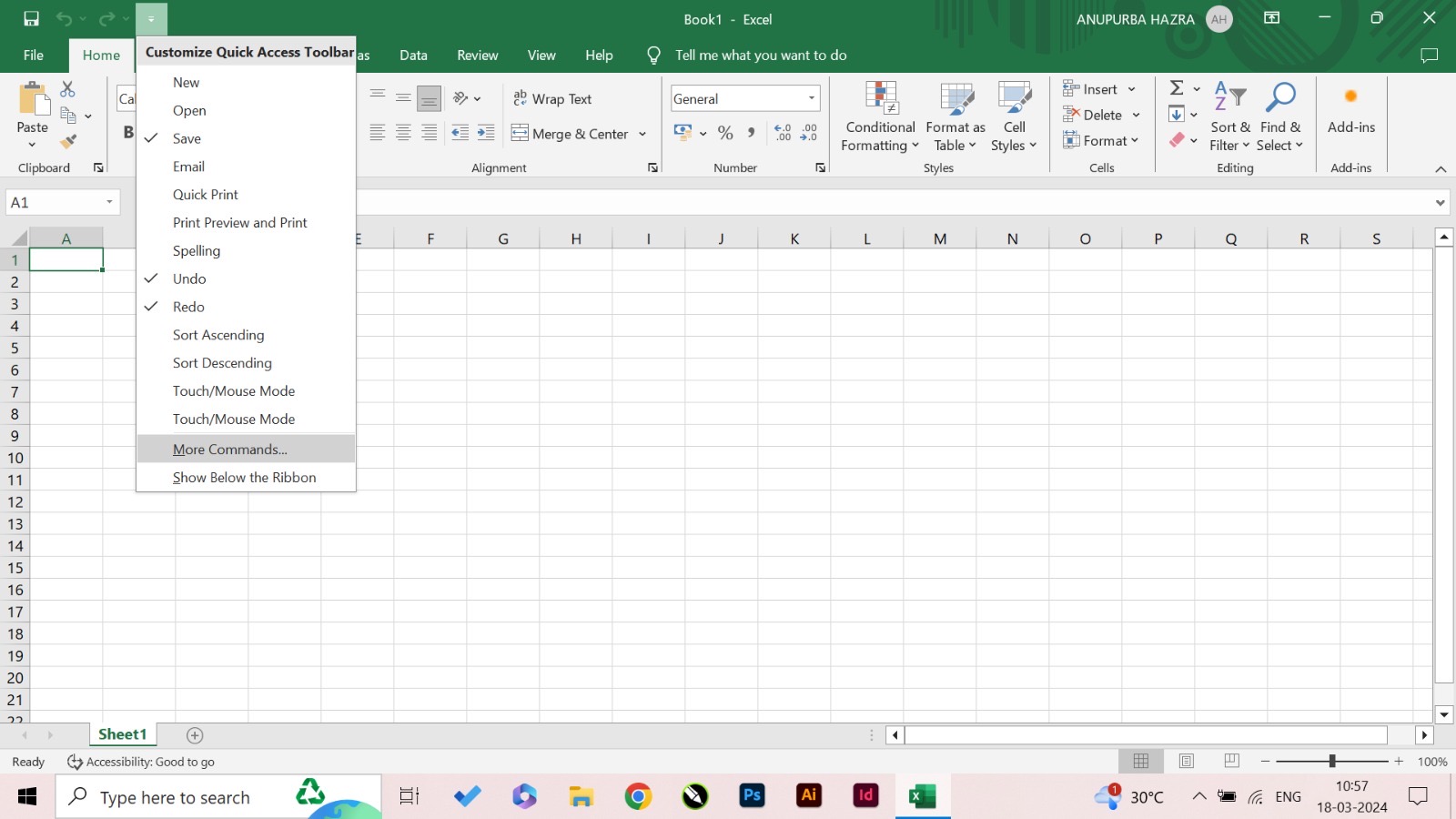
Source: MS Excel

You will see a dark gray horizontal line on the screen which locks the first row that you intended to freeze. You can move through the rest of the worksheet at your convenience.

However, if you want to unfreeze the selected rows and columns, then click on the freeze button again.

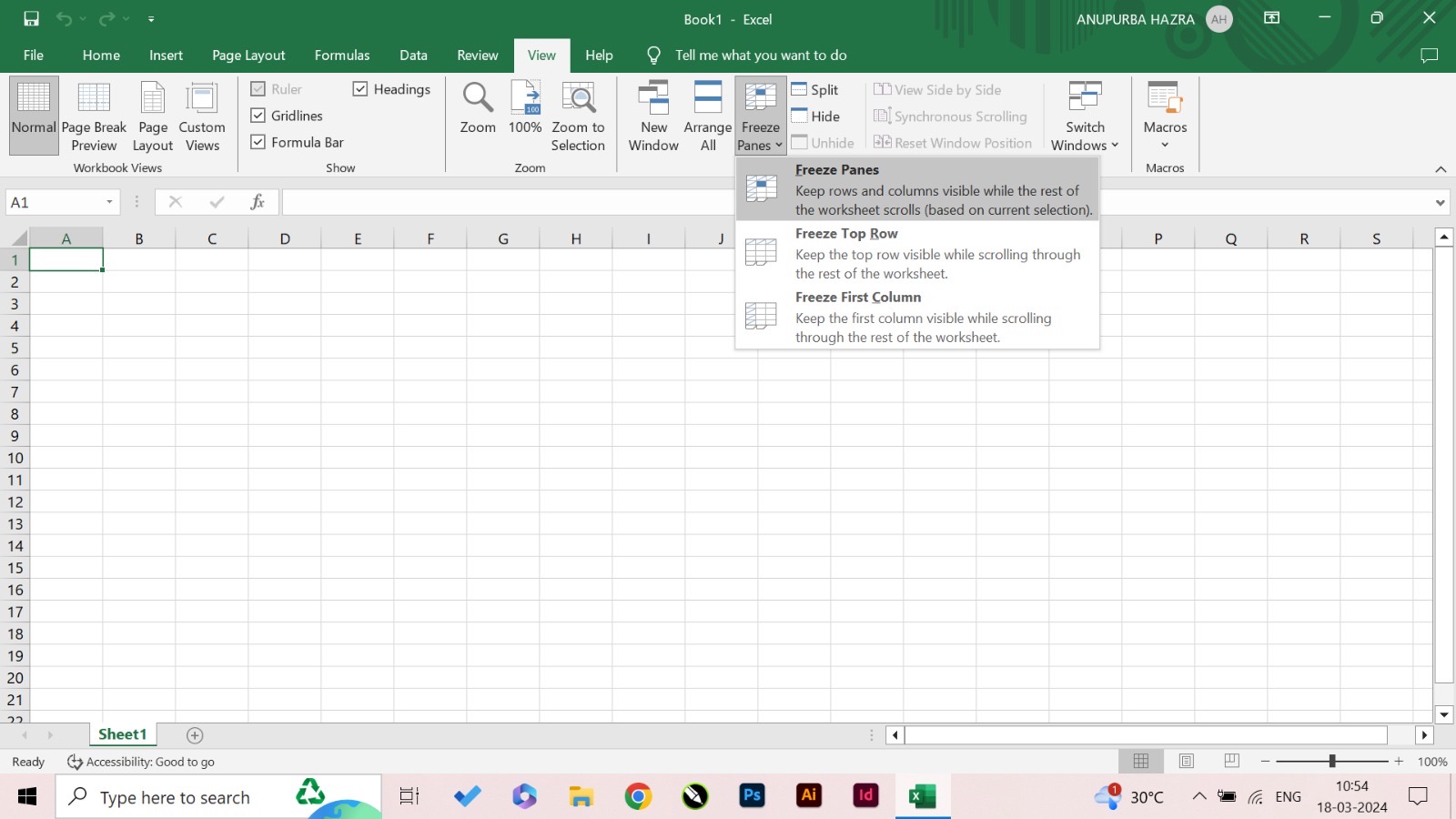
How to Unfreeze Panes in Excel?

If you want to unfreeze rows and columns or a cell in Excel, then follow the below-mentioned steps:

1. Move to the view tab in the windows section and select ‘freeze panes’.

2. A list will appear, from there choose ‘unfreeze panes’.

Source: MS Excel

This will ensure that the intended rows and columns will get unlocked. The dark gray horizontal line in the case of a row and the vertical line in the case of a column will be gone. Thus, ensuring that the panes are unfreezed.

Other Ways to Freeze Rows and Columns in Excel

Along with the option of freezing panes, Microsoft Excel provides further ways to lock particular areas of the spreadsheet. Following are the other alternatives.

Splitting Panes in Place of Freezing Panes in Excel

A very popular method of locking a cell in Excel is by dividing or splitting the spreadsheet into numerous parts. When you freeze panes, you can sustain and preserve the visibility of certain rows and columns, while traversing the worksheet.

However, when you split panes, you break the Excel window into either two parts or four parts. You can then move and access the intended sections separately and independently. Splitting the panes ensures that each section can work on its own and the cells in the other sections remain anchored when you navigate within the specific region.

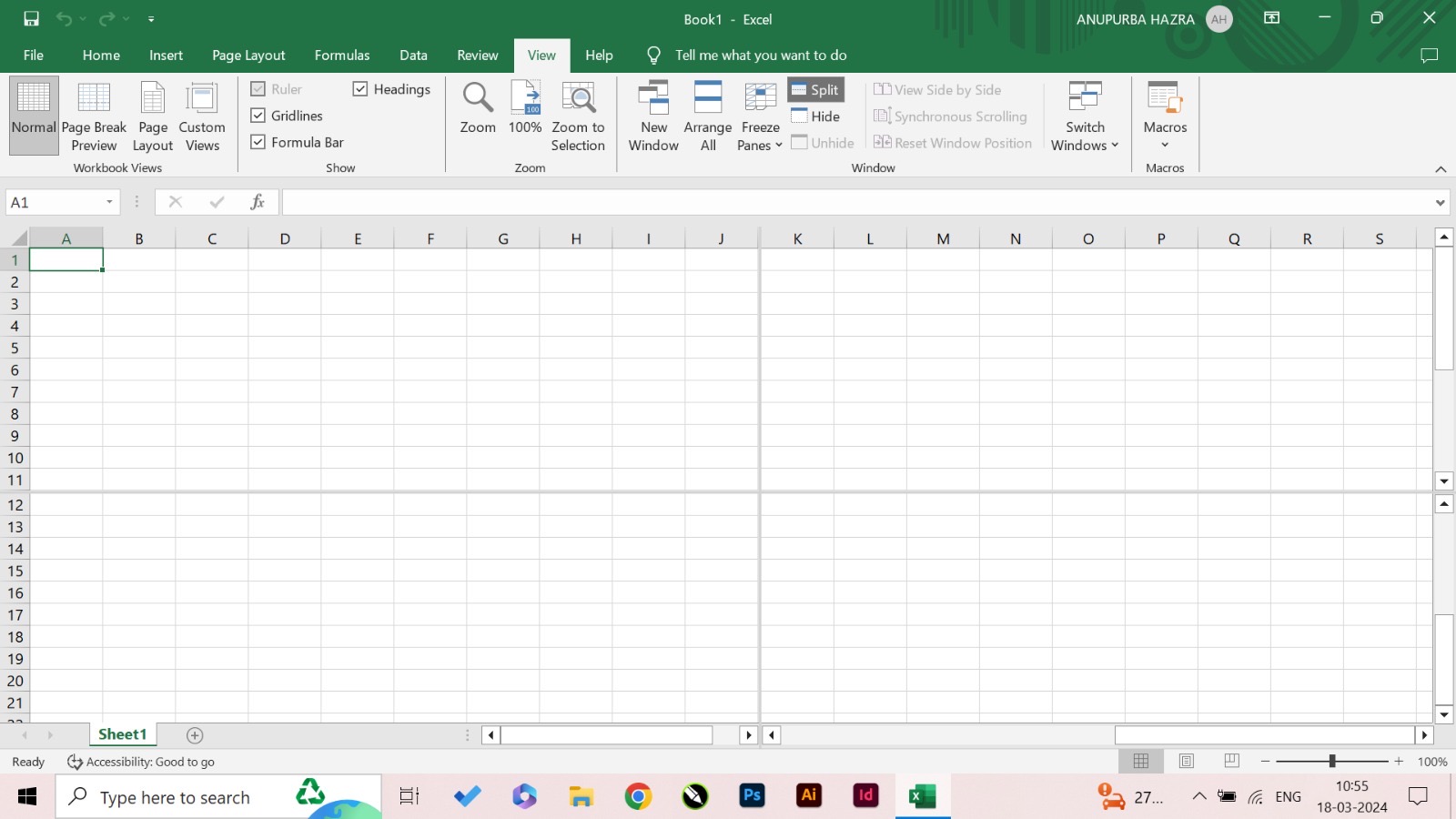
Source: MS Excel

This is how you can split panes in Excel:

1. Select the intended cell just below the row and right of the column that you want to split and opt for the ‘split’ option from the view tab.

2. If you wish to undo a split, click on the ‘split’ option again.
   

Using Tables to Lock the Top Row in Excel

To make sure that the row with the header stays intact at the top of the table, regardless of how you navigate down, convert a set into an Excel table and all the features and functions. You easily and quickly create a table in Microsoft Excel by employing the CTRL+T shortcut.

Print Header Rows on Each Page

If you want the top row or multiple rows to be kept the same and repeated on every page, you can use the print header row method. You can do so by following a few simple steps.

1. Move to the sheet tab and the rose that you want to repeat on top of the table on each page.

2. Select the ‘print title’ option and subsequently shift to the ‘page layout’ tab as well as the ‘page setup’ group.

3. Then insert titles for rows and columns on every page, and you’re done.

In Microsoft Excel, you can use this approach to freeze a row, multiple rows, one single column, or multiple columns, all at once.

Wrapping Up

All in all, freezing panes allow you to retain the access to crucial data and information. And, now that you know all about how to freeze panes in Excel, you’re all set to improve your data analysis tasks.

If you'd like to know more in-depth information about Excel spreadsheets and how they operate, you can check out upGrad's selection of engaging and dynamic courses. To succeed in your career, these courses can help you gain a deeper understanding of the subject.

Frequently Asked Questions

1. How do I freeze certain panes in Excel?

You can easily freeze panes in Excel by selecting the option that is most viable for you from the ‘View’ tab and the multiple selections available under the ‘Freeze Panes’ section. It provides a lot of options such as freezing the top row, multiple rows, the first column, multiple columns, or an entire cell.

2. What is the shortcut to freeze panes in Excel?

Apart from the standard measures, there also exists a freeze shortcut in Excel, which is selecting the Alt+W+F+F keys. This shortcut will freeze the first three rows and columns in your Excel sheet.

3. How do I freeze columns in sheets?

Just select the intended column that you want to freeze and click on the freeze option from the view tab and you can conveniently freeze columns in sheets.

4. How do I freeze the toolbar in Excel?

Move to the view tab in the windows section and select the option of ‘ribbon display’ at the top right corner. From there, choose any option and expand the river again.

5. How do I freeze panes vertically and horizontally at the same time?

To know how to freeze rows and columns in Excel at the same time, you have to freeze an entire cell. You can do so by moving to the view tab and selecting the option of ‘Freeze panes’.

6. How do you freeze multiple rows in Excel?

Select the row that is just below the concluding row that you want to freeze or simply choose the row’s first cell. Then move to the view tab and opt for ‘Freeze Panes’ and in this way, you can freeze multiple rows in Excel.

7. What is the shortcut key to freeze rows and columns in Excel?

The freeze shortcut in Excel with which you can freeze multiple rows and columns at the same time is the Alt+W+F+F function.

8. How do I freeze the first row and column in Excel?

To freeze the first row or first column in Excel, select the option of ‘Freeze panes’ in the view tab that is displayed on the Windows bar. Simply click on ‘Freeze top row’ or ‘Freeze Top column’ and scroll down to make use of the rest of the worksheet.