How To Highlight Duplicates in Excel

Many Excel users find duplicate entries while working in Excel. It can often offer a substantial barrier for users. Manually looking for duplicates can be time-consuming and cumbersome, especially for people inexperienced with effective procedures and algorithms. 

However, by applying dedicated formulas and leveraging certain methodologies, recognizing and highlighting duplicates can be simplified to mere seconds. 

In this blog, I’ll give you a brief method of instantly detecting and how to highlight duplicates in Excel, as well as arming users with the tools essential to handle this typical issue easily and quickly.

How to Identify Duplicates in Excel with Formulas?

Before you eliminate repeats in Excel, learn to recognize and highlight duplicates in your worksheet effectively.

Identifying Duplicate With the COUNTIF Function

To detect duplicates in Excel using formulae, you may use the following method using the COUNTIF function:

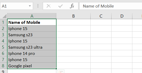
1. Suppose your data is in column A, beginning at A2.

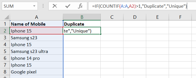
2. In an adjacent column (let's say column B), beginning from B2, put the following formula:

=IF(COUNTIF(A:A,A2)>1,"Duplicate","Unique")

1. Drag this formula down for all the cells in column B, matching your data range in column A.

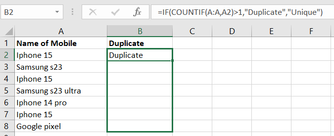
And now your duplicates are mentioned.

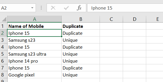
This formula validates each value in column A against the full column A. If the COUNTIF function returns a number larger than 1, it signifies the data is repeated elsewhere in the column. The formula produces "Duplicate" for duplicates and "Unique" for non-duplicates in column B. You may then filter or sort column B to quickly detect the duplicates. 

After that, you can select the duplicates and highlight them with the highlighter tool. This is a convenient solution - how to highlight duplicates in Excel.

Identifying Duplicate With the Conditional Formatting

1. Choose the column or range of cells you want to check for duplicates.

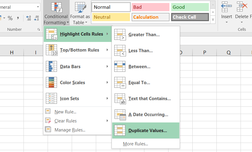
2. Proceed to the "Home" tab on the Excel ribbon and Click "Conditional Formatting" in the bar.

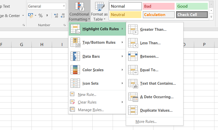
3. Select "Duplicate Values" from the submenu after choosing "Highlight Cells Rules" from the drop-down menu.

4. In the "Duplicate Values" dialogue box, you may specify how you wish Excel to format the duplicate data. You may maintain the default formatting or alter it according to your desire. Click "OK" to apply the conditional formatting.

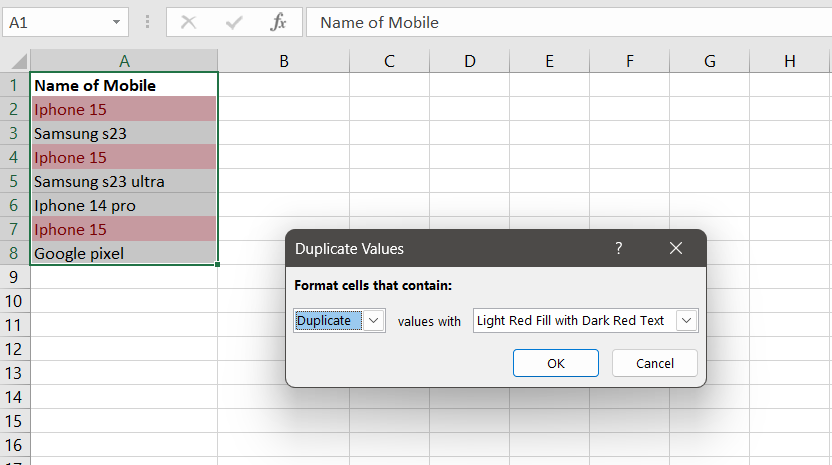
Excel will now find and highlight duplicate values inside the chosen range or column depending on the formatting criteria you defined. This makes it simple to find and manage duplicates in your Excel spreadsheet. This is one of the convenient solutions for how to highlight duplicates in Excel.

Finding Case-Sensitive Duplicates in Excel

Here, let me first explain to you what case sensitive is. It refers to a circumstance where text is interpreted differently depending on the capitalization of characters. In other words, uppercase letters are deemed separate from their lowercase counterparts. For example, in a case-sensitive comparison: 

"IPhone" and "iPhone" are regarded as distinct. 

Therefore, if you're looking for case-sensitive duplicates in Excel, it indicates that you want to detect instances when two or more cells have the exact text, but the capitalization of letters is different.

To identify case-sensitive duplication using a formula in Excel, follow these steps:

1. Suppose your data is in column A, beginning at A2.
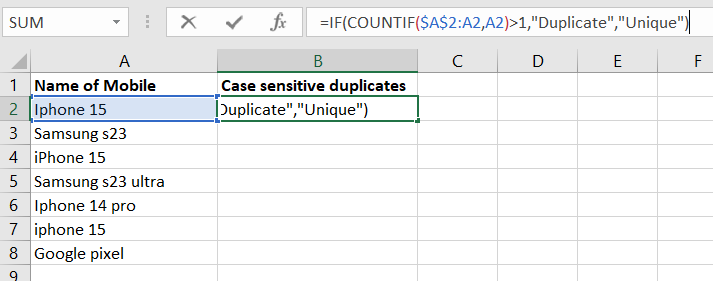
2. In an adjacent column (let's say column B), beginning from B2, put the following formula:

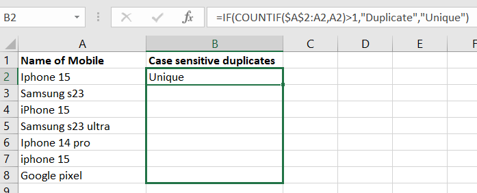
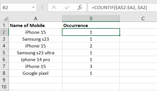
=IF(COUNTIF($A$2:A2,A2)>1,"Duplicate","Unique")

3. Drag this formula down for all the cells in column B corresponding to your data range in column A.

Here's what's happening:

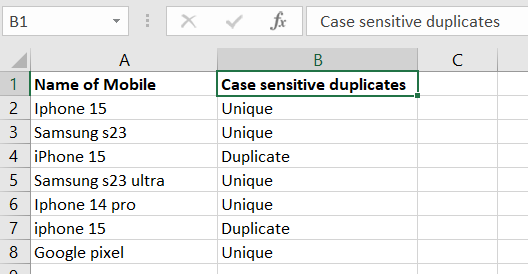
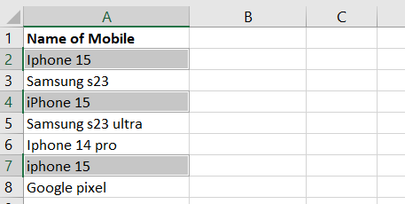
In cell B2, the formula checks whether "iPhone 15" occurs more than once in the range $A$2:A2. Since it's the first occurrence, it returns "Unique". In cells B4 and B7, "iPhone 15" occurs for the second and third time; hence it's recognized as a "Duplicate."

Similarly, the formula is applied to all cells in column B, showing whether the matching value in column A is a case-sensitive duplicate or unique. Next, you may use the highlighter tool to pick and highlight the duplicates. This is a convenient solution if you are looking for “How to highlight duplicates in Excel”.

Finding Duplicate Rows in Excel

Suppose your purpose is to dedupe a table consisting of numerous columns. In that case, you need a formula to check each column and detect only absolute duplicate rows, i.e., rows with the same values in all columns. 

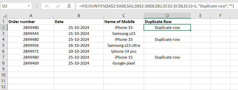
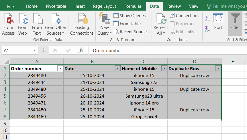
Let's analyze the following example. Supposing you have order numbers in column A, dates in column B, and ordered items in column C, you wish to discover duplicate rows with the same order number, date, and item. In order to test several conditions at once, I ll show you a duplicate formula based on the COUNTIFS function.:

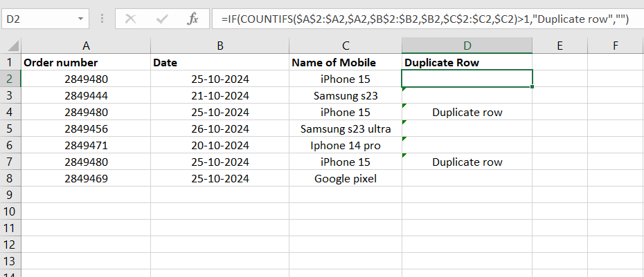
To search for duplicate rows with 1st occurrences, use this formula: 

=IF(COUNTIFS($A$2:$A$8,$A2,$B$2:$B$8,$B2,$C$2:$C$8,$C2)>1, "Duplicate row", "")

The screen below indicates that the algorithm locates only the rows with identical values in all three columns. For example, the same date as rows 1,4 and 7 but a distinct item and order number, so it is not identified as a duplicate row. Next, you may use the highlighter tool to pick and highlight the duplicates.

To show duplicate rows without 1st occurrences, make a little adjustment to the above formula: 

=IF(COUNTIFS($A$2:$A2,$A2,$B$2:$B2,$B2,$C$2:$C2,$C2)>1,"Duplicate row","")

There are numerous circumstances when you utilize these formulae to find your duplicated objects in Excel. Moreover, conditional formatting is the most straightforward technique to achieve these things in certain circumstances independent of the formula. Thus, you can explore Conditional Formatting in Excel more.

Counting Duplicates in Excel

Now that you have learned how to highlight duplicates in Excel, let’s move on to counting the overall number of duplicates.

Count Occurrences of Each Duplicate Record Separately

When you have a column with duplicated values, you may frequently need to know how many duplicates are present for each of those values.

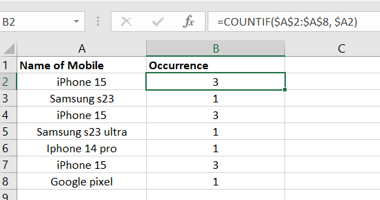
A simple COUNTIF formula may be used to determine how many times an entry occurs in your Excel worksheet, with A2 being the first and A8 being the last in the list:

=COUNTIF($A$2:$A$8, $A2)

If you want to figure out the first, second, third, etc. occurrences of every item, use the subsequent formula:

Counting the Total Number of Duplicates

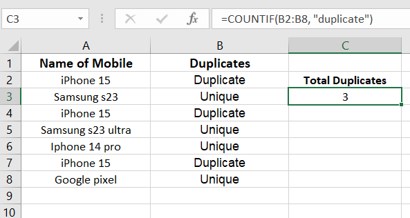
The best approach to counting duplicates in a column is to utilize any formula we use to find duplicates. Then, you may count duplicate values by using the following COUNTIF formula:

=COUNTIF(range, "duplicate")

Where "duplicate" is the term you supplied in the algorithm that locates duplicates.

So, these are how you may count the amount of duplicates quickly. 

Filter Duplicates in Excel

After learning how to identify and count duplicates, the next step is sorting them. To streamline data analysis, you might want to focus only on how to eliminate repeats in Excel . Here's a simplified procedure for filtering duplicates.

• Open your table, turn to the Data tab, and click the Filter option. Alternatively, you may choose Sort & Filter > Filter on the Home tab in the Editing group.

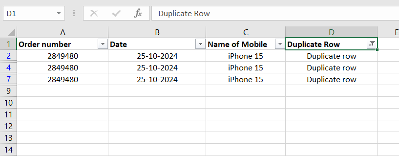
• After that, click the arrow Filtering arrow in the header of the Duplicate column and check the "Duplicate row" box to reveal duplicates. If you wish to filter out, i.e., conceal duplicates, pick "Blank" to display unique records:

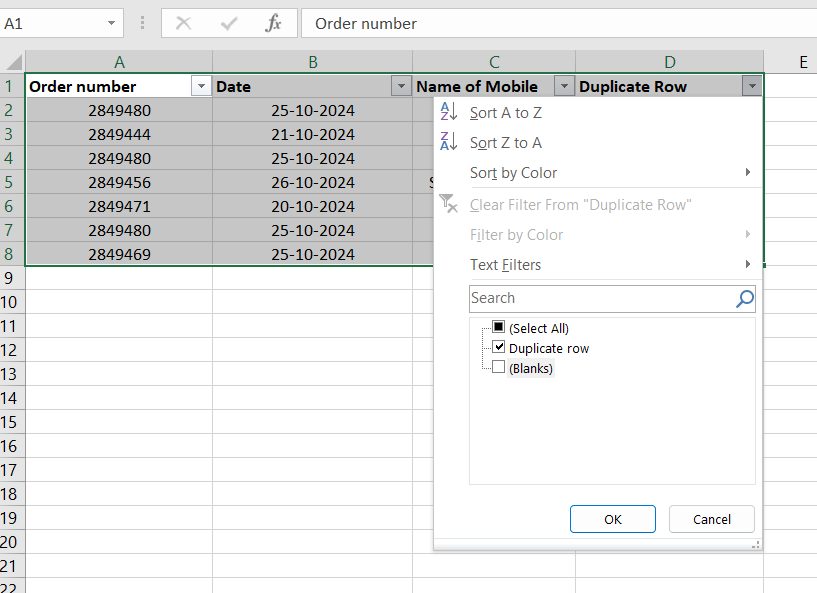
• Now, you may sort duplicates by the key column to group them for simpler examination. In this example, we may sort duplicate data by the Order number column.

Filtering duplicates in Excel automates the deduplication process, enhancing productivity in data-related tasks by swiftly identifying and removing duplicate records. The duplicate function in Excel hence, saves time and effort compared to manual data cleaning. It's particularly crucial before data analysis or report creation to ensure accurate and unique data points, leading to more credible conclusions. Additionally, it helps maintain data quality and improves overall efficiency in various data operations. Exploring advanced filter options in Excel is also recommended for better management of duplicates.

Remove Duplicates in Excel:

To delete duplicate lines in Excel, select them, right-click, and then choose Clear Contents. This deletes only the cell contents, leaving them empty. Alternatively, the same result may be obtained by choosing the duplicate filtered cells and then hitting the Delete key. To remove whole duplicate rows, first, filter the duplicates, select the rows by dragging the mouse across the row headings, right-click the selection, and choose Delete Row from the context menu.

Also, to learn more about these removal steps, you can use the formula to Delete Duplicates in Excel.

Highlighting Duplicates in Excel:

Select the filtered duplicates and click the ‘Fill Color’ button on the ‘Home tab’, then choose your desired color. You can also use built-in conditional formatting rules or create custom rules tailored for your sheet. Experienced users can create such rules based on the formulas that check duplicates. If you're not comfortable with Excel formulas yet, detailed steps are available in tutorials on how to highlight duplicates in Excel.

In Summary

Now that we have wrapped things up, I hope I have addressed all answers to the query, “How to highlight duplicates in Excel?” It's vital to identify duplicate entries to retain correct data rapidly. These practical strategies and shortcuts can improve your process, making it more straightforward to handle duplicates efficiently. 

If you want to upskill yourself to take your career to the next step, upGrad is your go-to learning platform. They offer the best online professional programs curated by industry experts and experienced professionals.

Frequently Asked Questions

1. How do I get Excel to highlight duplicates?

To learn how to highlight duplicates in Excel, you need to use conditional formatting or formulas to identify duplicates and highlight them.

2. What is the shortcut key for duplicate highlight in Excel?

There's no specific shortcut key for duplicate highlighting in Excel, but you can use conditional formatting or formulas.

3. How do you select all duplicates in Excel?

Select "Home" > "Conditional Formatting," then select "Highlight Cells Rules" > "Duplicate Values."

4. How do I find duplicates in Excel without removing them?

Find duplicates in Excel without removing them by using conditional formatting or filtering.

5. How do I find duplicates in Excel without deleting them?

Find duplicates in Excel without deleting them by using conditional formatting or filtering.

6. How do you filter duplicates in Excel?

Excel users can filter duplicates by selecting their data range, the "Data" tab, and "Remove Duplicates." When you choose which columns to search for duplicates in Excel, any duplicate rows will be eliminated, but the initial instance will remain. 

7. How do you highlight duplicates in Excel?

In Excel, highlight duplicates by selecting your data range, clicking the "Home" tab, selecting "Conditional Formatting," and then selecting "Highlight Cells Rules" > "Duplicate Values." 

8. What is the shortcut key to find duplicates in Excel?

To locate duplicates in Excel, use the shortcut Alt + H + L.