INDIRECT Function in Excel

Did you ever waste your time trying to create the perfect formula and feel content, only for it to collapse the moment a new column appeared?

I did. At that instant, all the references I so laboriously created pointed to something that did not exist. I started to feel completely overwhelmed by all the data. Then I found out about the INDIRECT function in Excel!

I could manage a large spreadsheet recording sales levels of numerous products across several regions with a click. There were also separate columns containing sales data for each region.

Want to build your sheet, too, like I did? Explore the detailed process here!

What is an INDIRECT function in Excel?

Picture this. You need to point to data in various cells or sheets. You'd usually type the cell ref like A1 or B23. But what if you want this point to be more changeable?

This is where the INDIRECT in Excel comes in handy! The tool takes a text, like "B12," and makes it a real cell reference that Excel can process.

The product? You can make cool sums that can shift based on other cell info.

But how would you use this? Say you're making a cash tracker. In one cell, you write "Income," and in another, "Rent." Then, with INDIRECT, you can make a sum that takes the amount from "Income" and cuts the amount from "Rent." Simple.

This is exactly what the INDIRECT function in Excel does. An online Excel course with certification can help you master this program quickly.

The INDIRECT formula

The INDIRECT function in Excel is a handy tool for making your formula change references independently. Here's the formula:

=INDIRECT(ref_text, [a1])

where

1. ref_text: This can be:

• A cell reference that holds the text stating which cell you want to look at (like A1 holding "B3").
• The text itself, if you put it in quotes (like "B3").

2. [a1] (optional): This bit tells the function if you're using the A1 style (which is the normal way) or the R1C1 style.

Let's try it out!

Let’s say you've got a table with titles at the top in row 1 and data below that. In cell B2, you want to show the number from the cell in row 2 under the "Sales" title.

Here's how to use INDIRECT function in Excel:

Step 1. In cell B2, punch in this formula:

=INDIRECT(A2&"2")

where

• A2 is titled "Sales" (if we say it's in A2).
• "&" glues the title "Sales" to the number 2 (which is row 2 here).
• INDIRECT reads "Sales2" as the spot to look at.

Step 2. Hit Enter.

Cell B2 will now show you the data from the second row that's under "Sales."

Features of INDIRECT function

Here's a quick look at what the INDIRECT function does:

• It's flexible: It lets you point to cells using text, which makes your formulas easy to change.
• It updates by itself: If the text in the cell you're pointing to changes, INDIRECT changes the link for you.
• It hides stuff: You can cover up tricky formulae with easy-to-read text.
• It works great with others: You can mix it with different functions to get changing figures.
  

How to use INDIRECT formula in Excel

Let’s look at how you can use INDIRECT easily.

Step 1: Grasping the rule

First, know the intricacies. As an INDIRECT rule, you will find the ref_text, which is a cell pointing to the text describing the cell you want to point to (for example, A1 pointing to "B3").

You can also find the actual text in quotes (like "B3"). You'll also find [a1], which is optional. (This sets the reference style (A1—default or R1C1).) For now, let's go with A1.

Step 2: Implementing it

Consider you have product names in column A and their prices in column B. In cell C2, you want to show the product price mentioned in cell A2. Here's the real use of INDIRECT function in Excel:

1. In cell C2, put the formula:

=INDIRECT(A2&"1")

2. Hit Enter.

The result?

Cell C2 will now display the price corresponding to the product name in cell A2. Cool, right? For more such skills, read up on an Excel tutorial specially crafted for beginners.

Examples of INDIRECT formula

Multiple examples exist outlining the versatility of this formula:

Using INDIRECT to set up a variable worksheet name

You got sales info for different months on sheets named "Jan," "Feb," etc. You aim for a formula in a main sheet to add up the total sales for any month.

Source: MS Excel

Step 1. In A1 (say), write the month's name to analyze (e.g., "Feb").

Step 2: In a different cell like B1, write this formula: =SUM(INDIRECT(A1&"!B:B"))

Result: When you change the month name in A1 (e.g., to "Mar"), the formula in B1 automatically updates to reference column B in the "Mar" sheet, giving you the total sales for March.

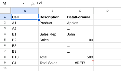
Using INDIRECT function in Excel for VLOOKUP

You have a product list on a separate sheet ("Products") with product names in column A and prices in column B. In another sheet ("Sales"), you want to use VLOOKUP to find the price of a product based on its name listed in the "Sales" sheet.

However, the sheet name "Products" might change in the future.

Source: MS Excel

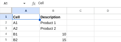
Step 1: In the "Sales" sheet, let's say cell A1 contains the product name you want the price for (e.g., "Product 1").

Step 2: In another cell (e.g., B1), enter the following formula:

=VLOOKUP(A1,INDIRECT("Products"!A:B),2,FALSE)

Result: When you enter a product name in cell A1 (e.g., "Product 1"), the VLOOKUP formula uses INDIRECT to reference the correct sheet ("Products"). It then searches for the product name in column A and returns the corresponding price from column B (10 in this case).

Using INDIRECT for multiple worksheets

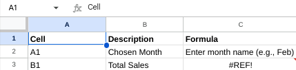
You're keeping track of sales in different sheets for regions like North, South, etc. You want a formula in a main sheet to get the total sales for any chosen area.

Source: MS Excel

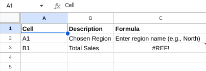
Step 1: Type the area name in A1, for example, "North". This tells the formula which sheet to focus on.

Step 2: In another cell, say B1, use this formula:

=SUM(INDIRECT(A1&"!B:B"))

Note: If you change the area name in A1 to "South", the formula in B1 updates to refer to column B in the "South" sheet, giving you the total sales for the South region.

Using INDIRECT with a dropdown list

You track expenses by category (Rent, Food) on separate sheets. You want a formula to find the total spent in any chosen category without manually typing the sheet name.

Source: MS Excel

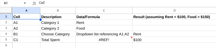
Step 1. List categories in column A (e.g., A1: Rent, A2: Food).

Step 2. Create a dropdown list in B1 referencing A1:A2 (Data tab > Data Validation > Allow: List, Source: =A1:A2).

Step 3. In cell C1, enter the formula:

=SUM(INDIRECT(B1&"!B:B"))

Using INDIRECT for locking cell reference

You have a table with things in column A and costs in column B. You want a way in cell C2 to show the cost for the thing in cell A2. But you don't want it to change if you add new rows or columns.

Source: MS Excel

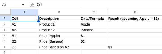
Step 1. Enter product names in A (e.g., A1: Apple, A2: Banana) and prices in B (e.g., B1: $1, B2: $2).

Step 2. Enter the formula with INDIRECT (Cell C2):

=INDIRECT("B"&A2)

Using INDIRECT function in Excel for fixed reference

You've got a list with item names in A and their costs in B. You need a way to put a rule in box C1 that will always show the cost of the item in box A1, no matter where you drag or copy that rule.

Source: MS Excel

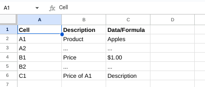
Step 1. In box A1, put the item's name (like "Apples").

Step 2. In box C1, write down the rule:

=INDIRECT("B1")

Result: This establishes a steady link to box B1, no matter where you shift the rule.

Using INDIRECT for a named range

You have a table with product names in A and sales figures in B. You want to make your named range more adaptable.

Source: MS Excel

Step 1. In column A, list different products while specifying their values in column B.

Step 2. Name this range “SalesData” covering B2 to B10, where the sales figures range.

Step 3. In another area, such as cell C1, input this formula:

=SUM(INDIRECT("SalesData"))

Result: It gives flexibility to your formula since you keep adding more data rows and expanding the named range, such as SalesData:B2:B15; everything will be calculated, including new data in the C1 formula.

Limitations of INDIRECT function

Despite its cool functionality INDIRECT, too, has its limitations.

• Hidden complexity: Even though convenient, INDIRECT can hide complex formulas behind easy-to-understand text, making it harder to see what's going wrong and fix it.
• #REF! errors: If the reference text is wrong (like a cell saying "B5" when there's no such cell) or goes beyond Excel's limits, it leads to the #REF! error.
• Closed workbook problems: Using INDIRECT to refer to cells in closed workbooks gets you a #REF! error. You might want to try VLOOKUP or INDEX/MATCH instead for getting data from outside.
• Simplicity is key: Sometimes, simple solutions like regular cell references or VLOOKUP/INDEX/MATCH might be better for basic referencing tasks.
• Dealing with errors: INDIRECT can be useful, but you should add error handling (like IFERROR) to prevent problems from spreading if something goes wrong.
  

Final thoughts

So here it is! You're all set to use the INDIRECT tool like an expert, making changeable links or even tricky fixed ones that don't move.

Want to boost your Excel game even more? Consider learning more with hands-on training from upGrad. They offer numerous certifications, beating complex equations, data study, and beyond. Go look at their site to find a course that suits you!

Till then, keep digging into Excel's magic and be surprised with what you can do with some fresh ideas and the perfect method. Enjoy your time with those spreadsheets!

Frequently asked questions

1. What is INDIRECT function in Excel with example?

The INDIRECT function changes the text to a cell link. Suppose you have items in A1:A10 and costs in B1:B10. In C1, put =INDIRECT("A1") to get the item name in A1, and bring the rule down to see names in A2, A3, and so on.

2. What is the INDIRECT Match function in Excel?

There is no "indirect match" rule. Yet, you can mix INDIRECT with MATCH for strong searches. Suppose you have a set of codes in A1:A10, and paired values in B1:B10. In C2, put =INDIRECT(MATCH("codeX",A:A,0)) to find the price linked with "codeX" (swap "codeX" with your real code).

3. What is the INDIRECT function in Excel filter?

INDIRECT doesn't work right with filters. But, you can use it for live rules for filters. For example, if A1 has "North," use =INDIRECT("A1") in your filter rules to only show lines where a region column fits "North."

4. What is INDIRECT function in Excel COUNTIF?

Like filters, INDIRECT isn't used right with COUNTIF. However you can use it for live ranges for tallying. Suppose your info begins in A2. Use =COUNTIF(INDIRECT("A2:A"&A1)) to count things from A2 to the line number in A1 (which can switch with user picks).

5. How do you use INDIRECT functions?

INDIRECT gets a text string as input. This string can be a cell tag itself (like "A1") or put right within quotes (like "B3"). INDIRECT then reads that text as a cell spot and returns the value or tag it holds.

6. What is INDIRECT and DIRECT function?

Excel doesn't have a direct function. But, INDIRECT is seen as an indirect link as it uses text to find the cell spot. On the other hand, a direct link just uses the cell tag itself (like A1, B23).