IRR Formula in Excel

Microsoft Excel is an excellent program to organize large groups of data. Of the many functions and formulae, I find the IRR formula in Excel to be the most useful. I work in finance, and the IRR formula in Excel helps me predict the profitability of my projects with ease. With IRR in  Excel, I can make informed decisions. 

In this tutorial, I will share my experience and teach you how to use Excel's IRR formula. You will learn the basics as well as advanced techniques like how to calculate XIRR in Excel. 

Understanding the fundamentals of IRR

Let’s learn the basics of IRR before you learn how the IRR formula in Excel works. I will briefly explain the internal rate of return (IRR) in finance. 

The IRR formula explained

The IRR is an important metric for evaluating investments and its profitability. The Internal Rate of Return (IRR) is the discount rate at which the net present value (NPV) of cash flows from a project equals zero. It represents the rate of return a project is expected to generate. 

The IRR formula involves setting the NPV of cash flows equal to zero and solving for the discount rate. Mathematically, it's expressed as the rate where the sum of the discounted cash flows equals the initial investment. 

Applying the IRR function in Excel

In this section, I’ll cover the exact IRR formula in Excel syntax for the internal rate of return Excel formula so you can harness the power of Excel's built-in internal rate of return calculator. Get ready to transform those cash flow projections into actionable investments using the IRR in Excel formula.

IRR syntax

The syntax of the IRR function is 

=IRR(values, [guess])

The required argument in the above syntax - values

This is the array or range of cells containing the cash flows of your investment. The cash flows must include at least one negative value, which will be your initial investment, and one positive value, which is returns.

The optional argument in the above syntax - It is a guess. 

You can provide or skip this number. It acts as the starting point for Excel’s calculation. If you skip it, Excel will use a default guess of 10%. 

Here is a step-by-step method with an example. 

Example explaining IRR formula in Excel

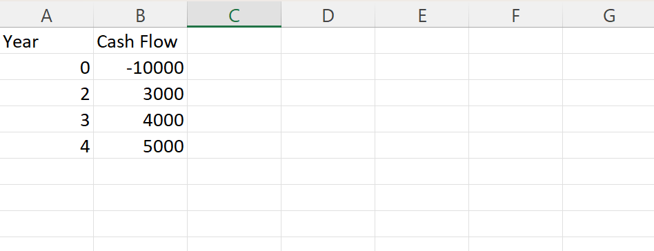
Let’s take an example where the initial investment is - ₹10000, and the cash flows are ₹3000, ₹4000, and ₹5000, respectively. How will you find the IRR using the IRR formula in Excel?

Step 1. Create a table in a new Excel worksheet to organize your cash flows. 

Step 2. List each year/period in the first column. In the second column, enter the corresponding cash flow for each period. 

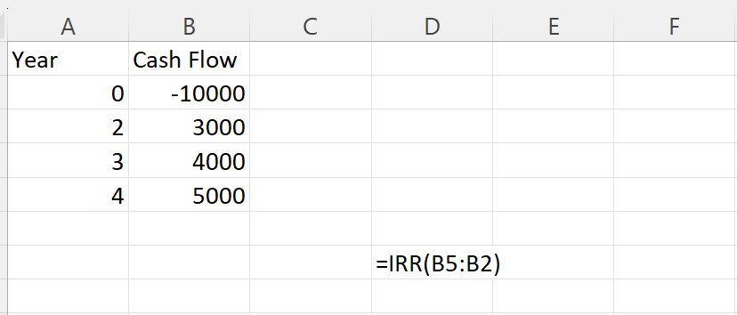
Step 3. Now, choose an empty cell where you want the IRR result to be displayed. In the chosen cell, type the following formula: replace B5:B2 with the actual range of your cash flow cells, including the initial investment = IRR (B5:B2). 

Step 4. Press enter. Based on the cash flow data, Excel will calculate and display the IRR for your investment.

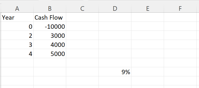
Step 5. The IRR result displayed is 9%. This percentage shows the growth rate of the investment. 

IRR calculation Excel example 

Now, let's see the IRR formula in Excel by exploring two practical examples. 

Example 1: Projecting cash flows of a new product launch

Let’s assume your company is considering launching a new product line of kitchen utensils. Let us see how IRR calculation can help you project cash flows associated with this venture:

Yearly Cash Flow (₹)

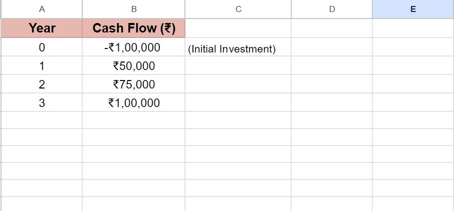
Step 1: Enter Your Cash Flows in Excel

Create a new Excel spreadsheet and list the cash flows for each year in a dedicated column (e.g., Column A). Label the first cell (A1) as "Year" and the subsequent cells (A2 onwards) with the corresponding years. In the next column (B2 onwards), enter the cash flow values for each year.

Step 2: Apply the IRR Formula

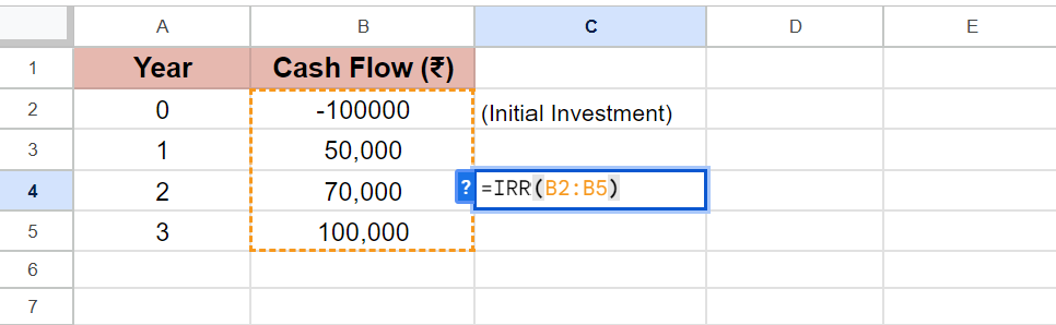
In a separate cell (e.g., C4), type the formula =IRR(B2:B4). This formula tells Excel to consider the cash flow range in cells B2 to B4 (inclusive) when calculating the IRR.

Step 3: Interpret the Results

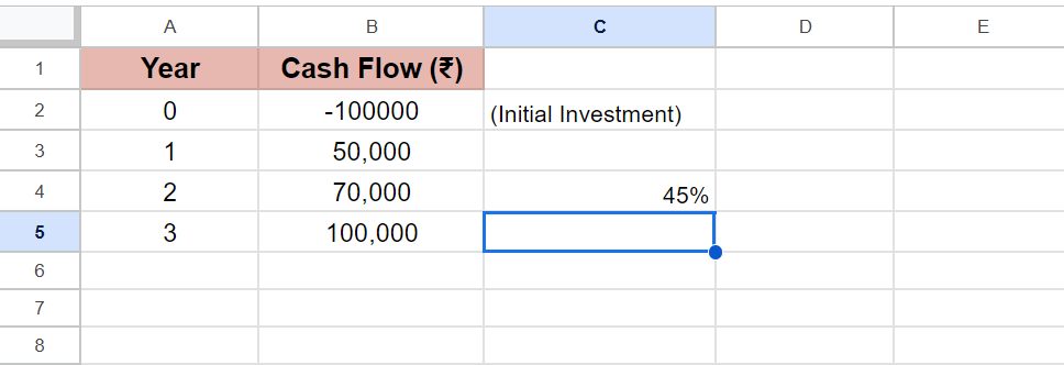
Hit Enter, and Excel will display the IRR which is 45% for this project. 

Beyond Basics - NPV, CAGR, MIRR, and XIRR

The IRR formula in Excel offers tremendous value. But what will you do when there are uneven cash flows? In this section, I will introduce you to Net Present Value (NPV), Compound Annual Growth Rate (CAGR), Modified Internal Rate of Return (MIRR), and the XIRR function. 

1. NPV in Excel

Net Present Value (NPV) is a core investment analysis technique that complements IRR. It determines the present-day value of future cash flows, discounted back using your desired rate of return (often your company's cost of capital). A positive NPV suggests the project generates value in today's terms, while a negative NPV means the opposite. 

Excel has a built-in NPV function, which, unlike IRR, directly incorporates your discount rate. This provides an apples-to-apples view if you compare projects of different durations.

Syntax: =NPV(discount_rate, value1, [value2],...)

Arguments:

1. discount_rate: The interest rate used to discount future cash flows.

2. value1, value2, ...: A series of cash flows occurring at regular one-period intervals (e.g., annually).

IRR vs NPV

IRR and NPV are closely related concepts in financial analysis. NPV calculates the present value of a project’s cash flows using a discount rate. 

NPV tells you whether an investment is profitable at a specific discount rate, while IRR tells you the break-even discount rate for that investment. Understanding both metrics gives you a complete picture of an investment’s potential using the built-in internal rate of return calculator Excel has. 

2. CAGR in Excel

Compound Annual Growth Rate (CAGR) reveals the average annual rate at which an investment has grown over a specified period. While not strictly an Excel function, you can calculate it using a formula. CAGR is helpful when analyzing past performance or smoothing out fluctuations in returns. Be aware that in some scenarios, IRR can approximate CAGR, but they diverge in some situations.

CAGR is not a built-in Excel function; therefore, the formula is:

 = (Ending Value / Beginning Value)^(1 / # of Periods) - 1

Arguments: 

1. Ending Value: Final value of an investment

2. Beginning Value: Initial value of an investment.

3. # of Periods: The number of periods over which the investment grew (e.g., years).

3. MIRR in Excel

Modified Internal Rate of Return (MIRR) addresses one of the inherent assumptions of the standard IRR function – it presumes that positive cash flows are reinvested at the same IRR rate. MIRR allows you to specify a separate reinvestment rate, giving it the potential to offer a more realistic picture, particularly for long-term projects. Excel has a built-in MIRR function to simplify calculations.

Syntax: =MIRR(values, finance_rate, reinvest_rate)

Arguments:

1. values: Series of cash flows, including initial investment (negative value).

2. finance_rate: The interest rate you pay on financing (i.e., your cost of capital).

3. reinvest_rate: The interest rate at which you reinvest positive cash flows.

4. XIRR in Excel

The XIRR function stands out when dealing with irregularly spaced cash flows. XIRR takes into account the specific dates on which each cash flow occurs. That is why the syntax for XIRR is also different from the standard IRR formula in Excel. The XIRR function is capable of calculating the exact time periods between cash flows. This leads to a more precise internal rate of return for uneven timeframes. 

Syntax: =XIRR(values, dates, [guess])

Arguments:

1. values: A series of cash flows.

2. dates: Corresponding dates for each cash flow.

3. [guess]: (Optional) An initial guess for the solution. The default is set to 10% in Excel. 

Choosing the Right Approach for Your Project - IRR vs XIRR vs MIRR

It is important to choose the best method for calculating and analyzing returns, taking your project’s cash flow characteristics into account. For most projects with an initial investment followed by a series of positive returns, the standard IRR formula in Excel is best. Otherwise, XIRR is the better option for dealing with uneven cash flow. MIRR is ideal when you have a clear reinvestment rate in mind.

Things to remember about the IRR formula in Excel

1. To get accurate results, your cash flow data needs to include at least one negative value (initial investment) and at least one positive value. 

2. If you encounter the #NUM! Error, here’s what might be happening: 

• Your cash flows might not have both positive and negative values. 
• The IRR calculation could not find a solution within the allowed number of tries. 

3. IRR is fundamentally linked to NPV. The IRR is the specific discount rate that results in an NPV of zero for your project’s cash flows. 

4. While optional, providing a ‘guess’ value in the IRR in Excel formula can sometimes help the calculation find a solution faster, especially for complex cash flow patterns. 

5. The standard IRR formula has limitations. Be aware of the reinvestment rate assumption and potential issues with multiple IRRs for unconventional cash flows. 

Summing It Up

From calculating IRR in Excel to understanding advanced applications like XIRR, hopefully this tutorial has equipped you with the knowledge to assess the potential returns of various projects confidently. 

The IRR formula in Excel is an excellent tool for financial analysis. For the most comprehensive decision-making, consider using it in conjunction with other metrics like NPV. To learn better experiment with the IRR calculation Excel provides, compare investments, and see how IRR can help you make data-driven decisions. 

If you are looking for even more in-depth financial modeling techniques and advanced Excel concepts, go for trusted platforms like upGrad. Their programs, designed in collaboration with top universities and industry experts, can further expand your expertise. 

Frequently Asked Questions

1. How do you calculate IRR on Excel?

You can calculate the IRR formula on Excel using the formula =IRR(values, guess). For detailed information, read the section - Applying the IRR function in Excel in the tutorial above.

2. How do you calculate levered IRR in Excel?

Calculating levered IRR in Excel requires more complex modeling. You will need to incorporate debt financing and its associated cash flows within your analysis with a combination of financial functions. 

3. How do you calculate IRR with example?

Refer to the section - Using the IRR formula in Excel in the tutorial above to learn how to calculate IRR with examples.

4. How do you calculate IRR quickly?

If you provide the ‘guess’ argument in the IRR in Excel formula, that can sometimes help Excel find the IRR faster. 

5. What is the IRR method?

The IRR method finds the discount rate that makes the Net Present Value (NPV) of an investment’s cash flows equal zero. It’s a way to estimate an investment’s potential profitability. 

6. How do you calculate IRR on a sheet?

Create a table of your cash flows in an Excel sheet, and then use the formula on Excel, specifying the cell numbers, to get the IRR in percentage.