For working professionals
For fresh graduates
- Study abroad
More
- Executive Doctor of Business Administration from SSBM
- Doctorate in Business Administration by Edgewood University
- Doctorate of Business Administration (DBA) from ESGCI, Paris
- Doctor of Business Administration From Golden Gate University
- Doctor of Business Administration from Rushford Business School, Switzerland
- Post Graduate Certificate in Data Science & AI (Executive)
- Gen AI Foundations Certificate Program from Microsoft
- Gen AI Mastery Certificate for Data Analysis
- Gen AI Mastery Certificate for Software Development
- Gen AI Mastery Certificate for Managerial Excellence
- Gen AI Mastery Certificate for Content Creation
- Post Graduate Certificate in Product Management from Duke CE
- Human Resource Analytics Course from IIM-K
- Directorship & Board Advisory Certification
- Gen AI Foundations Certificate Program from Microsoft
- CSM® Certification Training
- CSPO® Certification Training
- PMP® Certification Training
- SAFe® 6.0 Product Owner Product Manager (POPM) Certification
- Post Graduate Certificate in Product Management from Duke CE
- Professional Certificate Program in Cloud Computing and DevOps
- Python Programming Course
- Executive Post Graduate Programme in Software Dev. - Full Stack
- AWS Solutions Architect Training
- AWS Cloud Practitioner Essentials
- AWS Technical Essentials
- The U & AI GenAI Certificate Program from Microsoft
27. Columns in Excel
33. Count In Excel
49. Slicers in Excel
54. Solver in Excel
56. Macros In Excel
Cell References in Excel: Types, Usage & Examples
Are you still manually typing in your data and struggling with your formulas in Excel? Don't worry we have all been there, and done that, until I discovered cell references in Excel. With a simple cell reference, you can dramatically change how you work and how efficiently you complete your tasks.
To put it simply, Excel can find the values or data that you want the calculation to compute when you use a cell reference in a formula. This data can be any cell or range of cells on a spreadsheet. Excel offers three different kinds of cell references: mixed, absolute, and relative.
It's incredible how even a small adjustment to your strategy may increase your efficiency and save you time, which is often what's taught in Excel courses. Trust me, once you start using cell references in your work, you'll never return to your old ways!
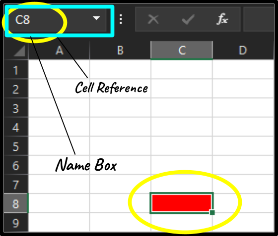
What Is a Cell Address or Cell Reference?
Suppose you have worked on Excel before you would already know that a spreadsheet is made up of cells. Each of those cells has a unique cell address or reference. When you click on a cell have you noticed how an alphabet or a combination of alphabets with the number is displayed on the side?
That is the cell reference in Excel and is used in most Excel formulas.
Source- Excel
The alphabet denotes the column that shows working on and the number identifies the row. Suppose you want to choose the 8th row of Column C, the name box will display “C8”.
Typing in the cell address of the cell in which you would want to add data or formulas in the cell box will redirect you directly to that cell in the spreadsheet. Not just one single cell, you can select as many cells, entire rows or columns as well.
When referencing data on a worksheet, data in various sections of the worksheet, or data on multiple worksheets within the same workbook, a cell reference can be used in formulae.
What are Range References?
A cell reference is referred to as "range" when it relates to more than one cell at a time. In Excel, a range reference is a collection of cells organized into rows or columns. For example, the range of cells A3 through C8 is indicated by the notation (=A3:C8). There is a colon used in between otherwise, Excel will return the standard error #VALUE.
How To Create A Reference In Excel?
In Excel, we can make a reference by following a few easy steps. They are as follows:
- Step 1: Choose the cell where the formula will be entered and type the equal to (=) symbol.
- Step 2: At this point, we have the option to click the cell directly or to type the reference straight into the formula box or chosen cell.
- Step 3: In the end, hit the Enter key.
For example,
You want to add the data in B2 and C2. We can enter =B2+C2 in D2 or the formula bar while selecting the D2 cell where we want our total data.
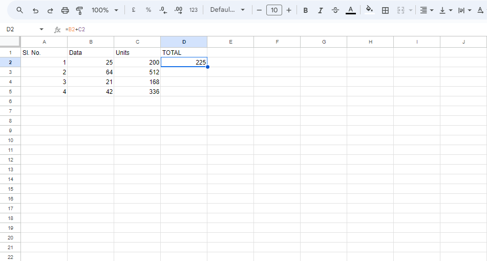
Source- Excel
On clicking Enter, the results will show.
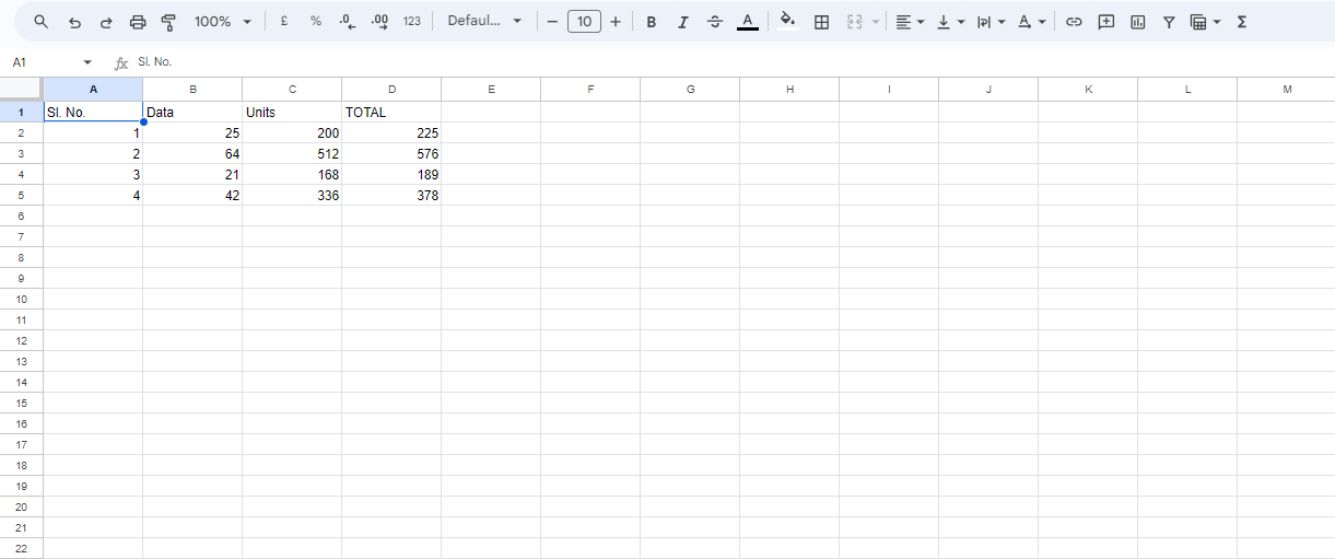
Source- Excel
How To Change A Cell Reference In A Formula?
Using the techniques below, we may modify the cell address in an existing formula.
- Step 1: You must first choose the cell that has the formula. Next, either double-click on the cell or hit the F2 shortcut key.
- Step 2: The new reference can be then chosen and entered into the formula. As an alternative, you can drag or choose the extra cells or cell range after selecting the reference.
Styles of Cell Reference
Excel offers two different styles of self-reference, A1 reference, and R1C1 reference. Allow me to elaborate on each point.
A1 Style of reference
We already discussed that each row and column is identified by a specific number or alphabet that is unique. These are termed the row heading and column heading which is primarily what A1 Style referencing refers to. So for example, a cell reference of D9 denotes that the particular cell lies in column D and row 9.
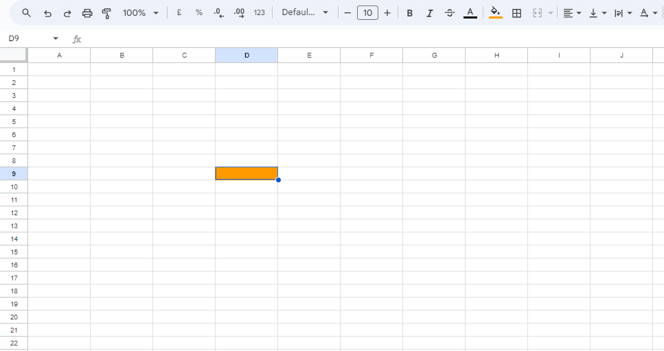
Source- Excel
This is the default reference style available in Excel for its users.
R1C1 Style of Reference
Apart from the default reference, R1C1 is another prominent cell referencing style. R1C1 is a style in which a cell in row 1, column 1 is designated by a number, indicating that this style recognizes both rows and columns.
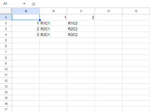
Source- Excel
If you want to shift from the default A1 style of referencing in Excel to the R1C1 style:
- Go to the File
- Click on options from the drop-down, and then click Formulas.
- Uncheck the R1C1 box.
Types of Cell Reference in Excel
Employing the correct addressing type will enable you to create complex formulas and improve your productivity while using Excel. Speaking of which, there are three main types of cell references in Excel: mixed, relative, and absolute cell references.
Here’s a detailed explanation of the same:
1. Relative cell reference
When you need to repeat computations across different cells or worksheets, you can use relative cell references. These references are altered when a formula is copied to another cell or worksheet.
They are identified by their lack of $ symbol in the row and column coordinates, such as A1 or B6:C12. Excel's cell addresses are all relative by default.
It's important to note that relative references are affected by the relative positions of rows and columns when they are moved or copied across numerous cells. Therefore, it's best to use relative cell references if you need to repeat the same computation over several rows or columns.
Example of relative reference in Excel
Let's assume that you are trying to multiply the data that is available in column B by 8 and see the result in column C.
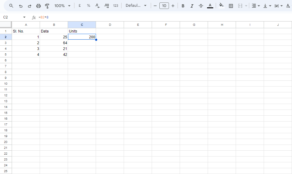
Source- Excel
For this, your formula will be, =B2*8
2. Absolute cell reference
A reference that has the dollar symbol ($) in the row or column coordinates, such as $A$1 or $A$1:$B$10, is considered absolute.
Adding the same formula to other cells does not modify the absolute cell reference. When you need to replicate a formula to other cells without altering references or when you need to do several computations with a value in a single cell, absolute addresses come in handy.
Example of Absolute Cell Reference Excel
After you have multiplied the data, you now want to multiply the values in column B by the value in column C2, enter the formula in D2 =B2 * $C$2.
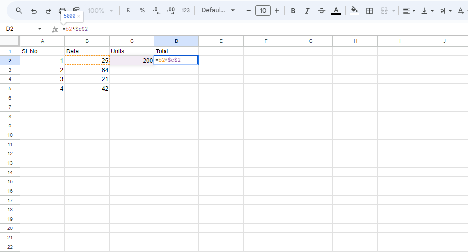
Source- Excel
You can then drag the fill handle to duplicate the formula along the column.
When copying a formula, the relative reference (B2) will shift according to the relative location of the row, while the absolute reference ($C$2) will remain locked in place on the same cell.
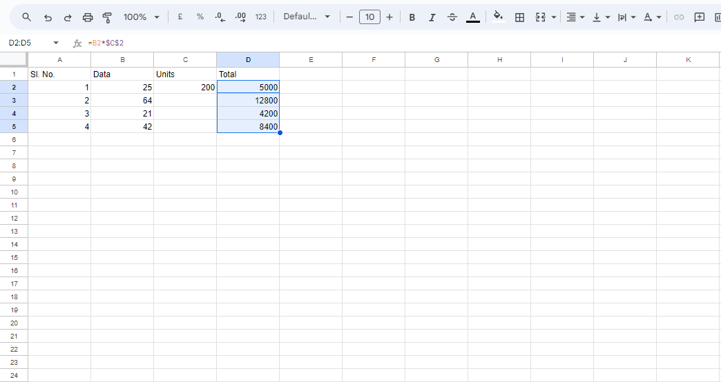
Source- Excel
3. Mixed cell reference
It combines absolute and relative references wherein, one relative and one absolute coordinate are present in a mixed cell reference. Dollar signs are appended to either the letter or the number in an Excel mixed reference excel, for instance, $C6 or C$6
In many cases, just one coordinate—a column or row—needs to be corrected.
Various complicated equations can be simply carried out with the help of mixed cell reference because it cuts down on the process of having to do each calculation manually and uses the available resources of both relative and absolute references in Excel.
Example of mixed reference Excel
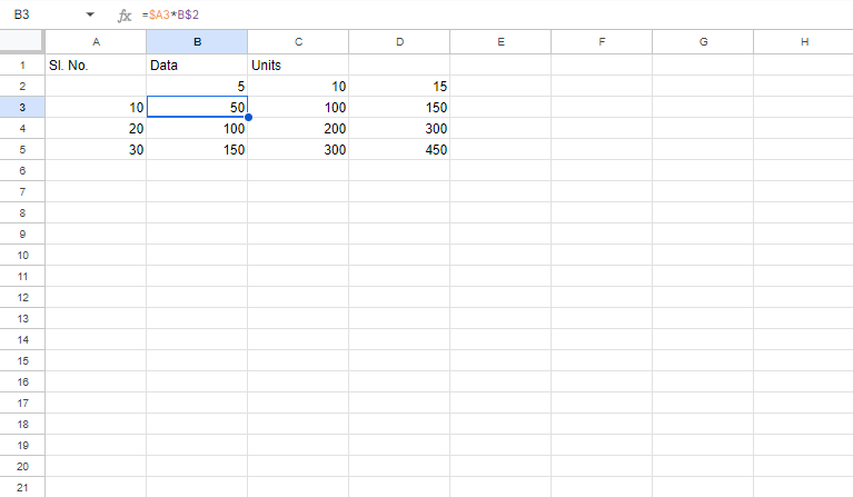
For instance, you would enter the following formula in column B3, copy it down and to the right, and multiply a column of numbers (column A) by three distinct numerals (B2, C2, and D2).
=$A3*B$2
To ensure the formula always multiplies the initial values in column A, lock the column coordinate with $A3. For the multiplier, lock the row location in B$2 since it's in row 2. Since the multipliers are in different columns, keep the column coordinate relative and adjust the formula accordingly.
As a consequence, a single formula is used for all computations, and it appropriately adjusts for each row and column where it is used.
Source- Excel
Switch Between Different References
So far we understood the major styles and types of referencing in Excel. However, you might be required to change the cell reference and operate a different formula to accommodate changes.
This can also be done with a simple switch between the different reference types.
To switch between reference types:
- Select the cell in which the formula lies
- Go to the formula bar
- Press the shortcut F4 key to change the reference type.
You can do this or you can also try a different method. By selecting the cell with the formula you can either manually press delete on the dollar ($) symbol or add a dollar symbol ($).
In Summary
So, to conclude this fun tutorial, I’m just going to assert the importance of cell references in Excel. As a key element for carrying out formulas and other functions with the data in Excel, you can use them to perform task charts and also carry out other relevant Excel commands. However, be mindful of what type of reference you use because it will depend on the category.
Employers of major companies all around the world are vastly recognising the need for employees who can organize, calculate and draw inferences from data quickly and accurately. So if you want to get ahead of others and enhance your skills, upGrad has over 500 courses on offer where you can learn from the best, get degrees and certificates and be a master in Excel and beyond.
Frequently Asked Questions
- What are the 3 types of cell references in Excel?
There three types of cell references in Excel, are relative cell reference, absolute cell reference, or mixed cell reference. All these three types of references can be used for carrying out specific tasks and have unique characteristics when being copied or located elsewhere.
- How do you set a cell reference in Excel?
To set a cell reference in Excel:
- Click the cell for the formula.
- In the formula bar, type "=".
- Choose the desired cell or range.
- Press Enter after selecting.
- What is an example of a relative cell reference in Excel?
Let's assume that you are trying to multiply the data that is available in column B by 8 and see the result in column C. The formula is =B2*8. This type of reference comes in handy when similar or repetitive calculations need to be done across various columns and rows in the spreadsheet
- How do you fix cell references in Excel?
You may "lock" or fix the original cell reference to keep it the same when you replicate it by placing a dollar sign ($) in front of the cell and column references.
- What is a cell reference from a cell value in Excel?
Cell values are the data entered into spreadsheet rows and columns, while cell references identify where the data is located. References can be specific or span a range of cells. Excel operations rely on these references and formulas to manipulate cell values.
- Where is the f4 key in Excel?
You will find the F4 key on the top row of your keyboard.

Author|14 articles published


upGrad Learner Support
Talk to our experts. We are available 7 days a week, 9 AM to 12 AM (midnight)
Indian Nationals
Foreign Nationals
Disclaimer
1.The above statistics depend on various factors and individual results may vary. Past performance is no guarantee of future results.
2.The student assumes full responsibility for all expenses associated with visas, travel, & related costs. upGrad does not provide any a.


