Pivot Table in Excel

One of the most powerful MS Excel features is a pivot table. When I first started using them, I'll admit, they seemed a bit daunting. But once I got the hang of it, I realized just how indispensable they are for summarizing and analyzing complex data.

In this article, I'll guide you through the ins and outs of this tool, breaking down the process step by step so you can wield a pivot table in Excel with confidence and expertise.

What is a Pivot Table?

Learning about the pivot table in Excel is crucial to Excel training and stands out as one of the most powerful and indispensable features of this spreadsheet software. Its primary function? Wrangling large volumes of data into a structured table format. Without it, this task could be a tedious ordeal, but with the pivot table's help, it's swift and effortless.

What sets the pivot table apart is its ability to neatly organize chaotic data, making insights readily accessible. With a simple rearrangement, data can be shifted and grouped to reveal different perspectives and answers. Hence, its name – pivot table – implying its capability to pivot or rotate data seamlessly, providing users with versatile analytical tools.

What is The Use of Pivot Table in Excel?

The pivot table in Excel is invaluable for summarizing, analyzing, displaying, and organizing extensive datasets. They streamline complex information, making it more manageable and comprehensible. With pivot tables, users can efficiently address intricate data queries and uncertainties, facilitating smoother decision-making processes and insightful analysis.

A pivot table can be used in the following circumstances:

• When the final sales total of different products is compared with each other a pivot table is needed.

• A pivot table is used while merging similar data.

• It is also used while noting down the data of various employees from different departments.

• A pivot table can also add a default value to any empty Excel cell.

• Taking out different sales percentages from the total value.
  

Various Components of a Pivot Table

A holistic understanding of pivot table in Excel also includes knowing about its components. I have explained the various components of a pivot table here:

Pivot Cache

After creating a pivot table in Excel, the application automatically starts to record the data inserted in the pivot table and keeps them stored in its memory. This backup data is referred to as the pivot cache. When the point of view of a pivot table is changed, Excel uses this pivot cache to calculate the final result or output in no time.

Value Area

The cells of MS Excel that hold the calculations in a pivot table are known as the value area.

Rows Area

The rows that exist just adjacent to the value area are known as the rows area of a pivot table in Excel.

Column Area

A value area in a pivot table has various headings that distinguish between various data. This heading area is located just above the value area and is known as the column area.

Filter Area

The filter area is an option available in a pivot table that filters a particular data that the user wants to calculate.

Pivot Table Example

There are numerous circumstances where a pivot table is required to ease down work and calculation. Here are the top three instances or examples when a pivot table is required in Excel:

1. Creation of a Budget

One of the most important tasks of a pivot table is to track the budget, it can be a personal money budget or the budget of a big business firm. It helps to track expenditures, gives you various ideas about saving money, and eases complicated budget calculations. A budget pivot table must contain the following heads:

1. Deposit of Money
2. Withdraw of Money
3. Date of withdrawal and deposition
4. Reasons for withdrawal as well as deposition of money

2. Making of a PTO Tracker

Paid time off or PTO is a time when an employee takes a leave from his work and is still getting paid for those days when he did not work. The PTOs of a company are tracked and supervised by HR. Hence, to assist an HR with this tracking a pivot table in Excel comes into rescue.

The HR can track all the PTOs of every employee by simply putting them together inside a pivot table. Data on various leaves like sick leave, overtime hours, hours of PTO, etc are tracked and calculated minutely with the help of a pivot table.

3. Closely Analyzing a Campaign Performance

A pivot table allows a user from a business company to track the performance of the last campaign by vividly studying regional success and acceptance.

How to Add Pivot Table in Excel?

You might be wondering how to create pivot table in Excel. There are a few simple steps that you need to follow, however, it might be quite intimidating for a beginner. Here I have discussed each step in detail:

Insert Table

To insert a pivot table in Excel you must follow these steps:

• You need to select any cell in the Excel worksheet.

• After that, you must click on the insert table. Where you will find the group known as tables.

• From the table, you can insert a pivot table in the worksheet.

• After clicking on the pivot table option a dialogue box will appear.

• In that dialog box, MS Excel automatically fills up the range box by analyzing the data that is already there in the worksheet.

• In the second option, you can set the location of your pivot table according to your choice.

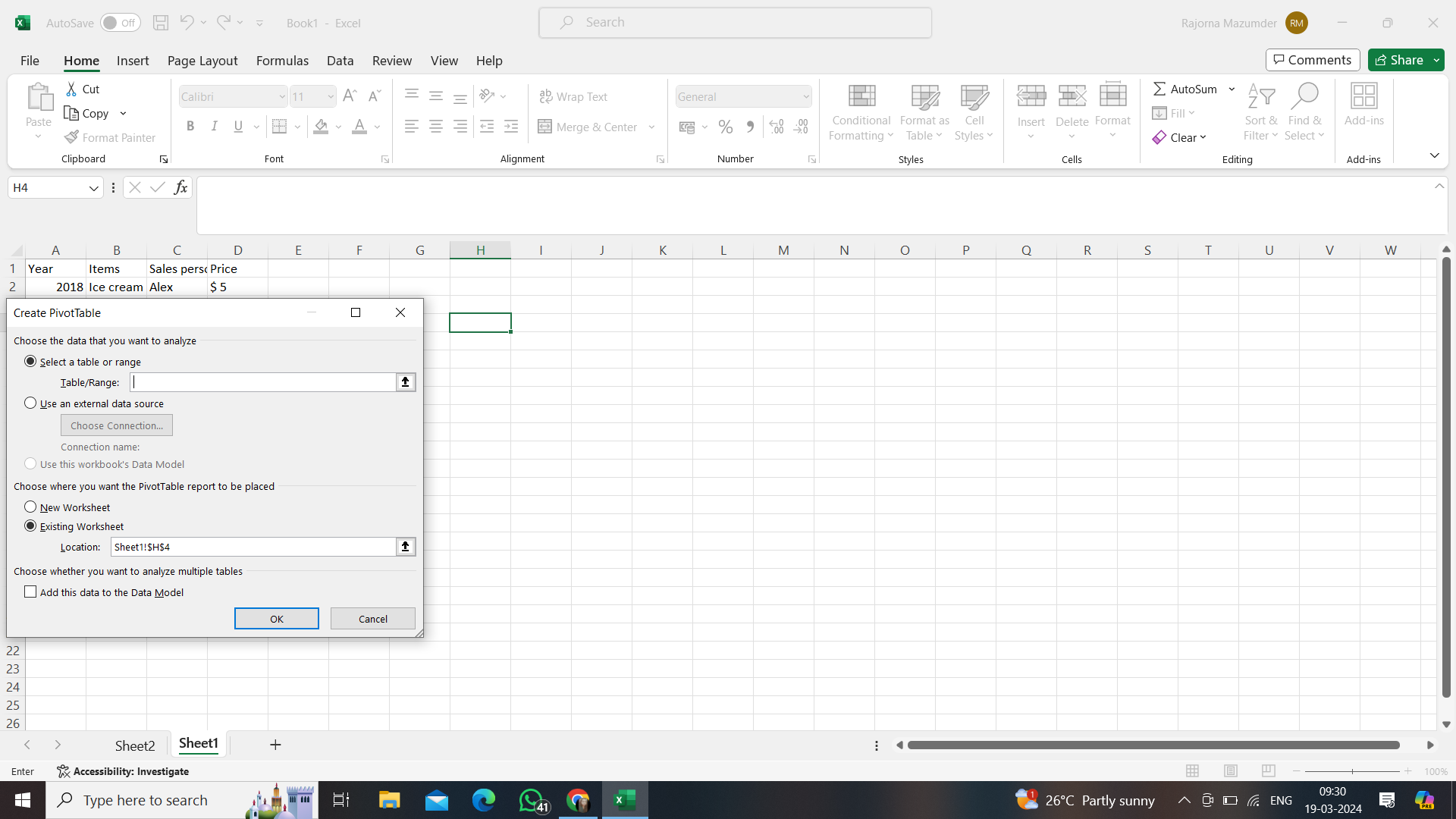
Source: MS Excel

• In the last step after filling up all the boxes, you should click ‘OK’ to insert the pivot table in the Excel sheet.

Source: MS Excel

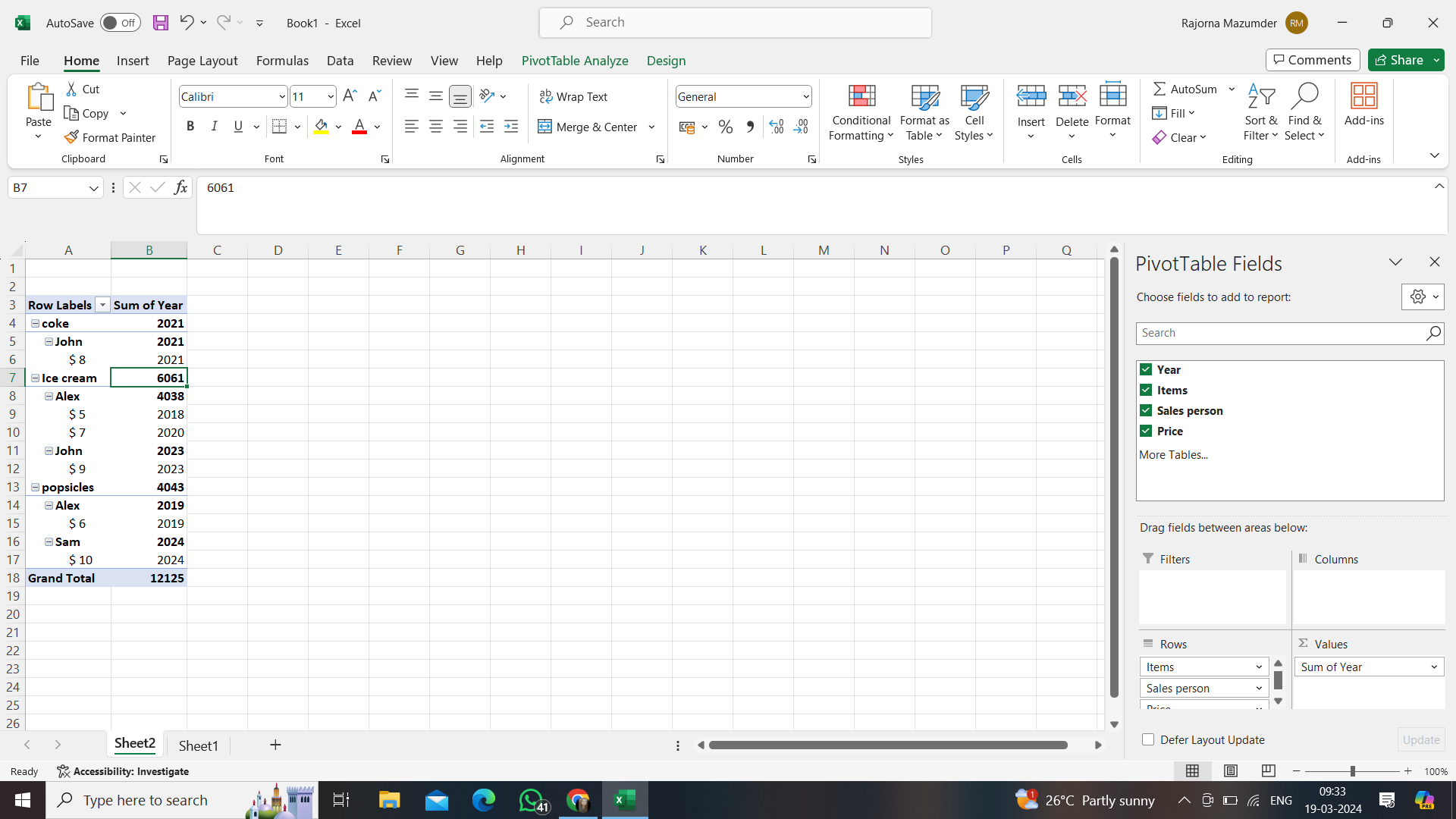
Two-Dimensional Pivot Table

You can easily create a two-dimensional pivot table in Excel by moving different fields to different areas like you can move the region section to the column area or sales data to the vale area. This creates a new point of view and thus you can easily create a two-dimensional pivot table.

Data Grouping in Pivot Table

MS Excel has a feature that allows in grouping of the pivot table data in various segments so that all the calculations can be easily implemented and distinguished from other data. If you want to create a separate group then you have to follow these steps:

• In the first step, you have to select the data that you want to group together.

• After selecting the data you need to press the right-click and a dialogue box opens.

• There you can find the group option. So you need to click on that.

• Then the data of that pivot table is finally grouped together.

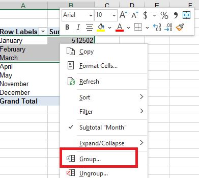
Source: MS Excel

Percentage Contribution

MS Excel has a feature where you can add percentage contributions in various forms. To add a percentage contribution you need to follow these steps:

• In the first step, you have to right-click on the pivot table where many options will appear.

• Then you need to click on the ‘Show Values All’ option after which more options will appear.

• Then you need to click on the ‘% of Grand total’ to add percentage contribution in the pivot table.

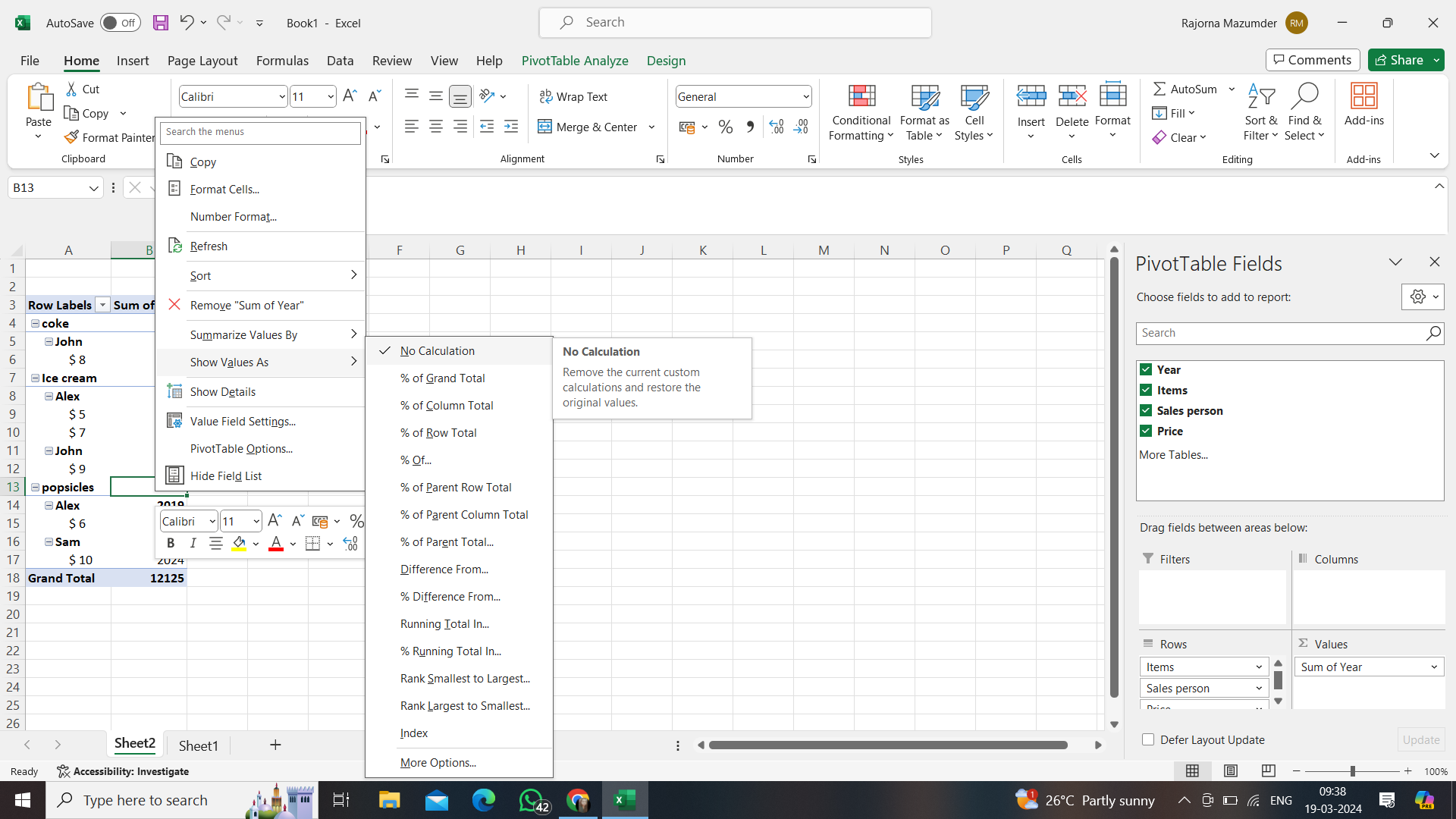
Source: MS Excel

In Conclusion

In short, a pivot table in Excel is a super handy tool for making sense of complicated data. They might seem tricky at first, but once you get the hang of them, they can really help you understand your data better. Whether you're new to Excel or a pro, learning how to use pivot table in Excel can make your life a whole lot easier.

Excel skills are mandatory especially if you are pursuing data science or analysis as a career. upGrad not only offers expertly-designed Excel tutorials and courses, but also other relevant data science courses.

Frequently Asked Questions

1. What is a Pivot Table in Excel used for?

The pivot table in Excel is used to summarize and analyze huge data which is difficult to calculate.

2. How to create a Pivot Table in Excel?

If you want to create a pivot table in Excel you must go to the insert tab. There under the table group option, you can insert a pivot table in your Excel worksheet.

3. What is the Pivot Table formula?

In Excel, there isn't a specific "Pivot Table formula" per se, as pivot tables are created using the PivotTable tool and not formulas.

4. What is pivot chart in Excel?

MS Excel has many built-in features, pivot chart is one of those features. The main function of a pivot chart is to summarize the data that are available in the pivot table.

5. What is the command for PivotTable in Excel?

The command for creating a new pivot table in a new Excel worksheet is Fn+F11.

6. What is pivot formula in Excel?

There isn’t one. However, some common Excel formulas used in pivot tables include SUM, AVERAGE, COUNT, and IF, among others. These formulas allow you to calculate values based on the data in your pivot table and customize the analysis to suit your needs.

7. What is the shortcut key for PivotTable?

The shortcut for creating a new pivot table in a new Excel worksheet is Fn+F11. And if you wish to create a pivot table in the existing worksheet then you need to press Alt+F1.

8. What is the difference between pivot and pivot table?

Pivot in MS Excel is a simple feature that refines or remolds the data and value. Whereas, a pivot table is an extremely powerful feature that summarizes and calculates the value of very complicated data.