How to Use SUMIFS Function in Excel

The SUMIFS function in Excel, for lack of better words, is the core function of Excel sums. It serves as a fundamental tool for calculating sums based on specified criteria. But it can be a little confusing if you’re new to Excel. I’d suggest going through an Excel tutorial for beginners.

Now, let’s jump straight into how to use SUMIFS function in Excel. Let’s get started!

What Is the SUMIFS Function in Excel?

For starters, the SUMIFS function is a pre-existing function in Excel that allows you to add up the range based on one or more TRUE/FALSE conditions, including an Excel SUMIFS date range.

To start with, consider three criteria:

criteria1, criteria2, and criteria3

These are the ranges, and the work happens using these conditions:

• If a number is greater than another one (>)
• If a number is smaller than another one (<)
• If a text/number is equal to another (=)

Finally, to sum these, you use this function:

[sum_range]

Formula for Excel SUMIFS

Using the ranges and conditions stated above, you enter this syntax:

“SUMIFS ( sum_range, criteria_range1, criteria1, [criteria_range2, criteria2, criteria_range3, criteria3, … criteria_range_n, criteria_n] )”

where

• sum_range: cells to add up
• criteria_range1: range of cells that you want to apply the first criteria (criteria1) against
• criteria1: for determining the cells that need to be added
• criteria_range2, criteria2, and so on: the additional ranges alongside the criteria you’re working with

Note: Under all circumstances, you can only apply this to up to 127 criteria pairs, better known as range. Also, check out the Excel free online course with certification to track the scope of Excel skills.

Remember:

1. SUMIFS is solely represented by a numerical value.
2. All rows and columns in your function should be of the same criteria_range argument and sum_range argument.
   

How to Use SUMIFS Function in Excel

You have your cells and your ranges. Now, all you need to do is define the criteria.

Note that Excel supports two kinds of ranges: logical operators (>,<,<>,=) and wildcards (*,?,~).

We have our syntax:

=SUMIFS(sum_range,range1,criteria1) // 1 condition

=SUMIFS(sum_range,range1,criteria1,range2,criteria2) // 2 conditions

The first argument here (sum_range) points to the range of cells to sum.

The second (range1), is the range to which the first condition will be applied.

The third argument (criteria1) is the basic condition that you’ll apply to (range1). Here, you will use logical operators.

But before you ask Excel to work for you, keep in mind:

• All conditions should be TRUE for it to be included in the final sum.
• All the criteria should include logical operators when needed.
• All ranges must represent the same size failing which the SUMIFS function, unequivocally, returns a #VALUE! Error.
• Every new condition will work only with a separate range and criteria.
  

Example of SUMIFS Function

Sum time with SUMIFS

Let’s say you have a data table with employee IDs, project names, and times spent working on each project. You want to calculate the total time each employee spent on a specific project.

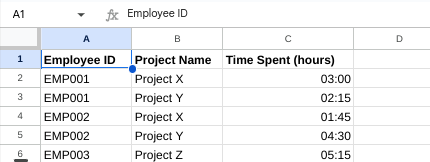
=SUMIFS(C:C, A:A, "EMP001", B:B, "Project X")

where

• C:C: is the range containing the time spent values (hours)
• A:A: is the range containing employee IDs
• "EMP001": is the criteria for the employee ID
• B:B: is the range containing project names
• "Project X": is the criteria for the project name

Result: This formula will add up the time spent by employee "EMP001" on "Project X" which in this case is 3:00 hours (assuming cells are formatted for time).

Sum for cells containing specific text

This is the one for you if you wish to learn how to use SUMIFS function in Excel with a specific test.

You have a sales table here with columns for Product (text), Category (text), and Price (number). We want to find the total sales for Shirts in the Clothing category.

=SUMIFS(Price_Range, Category_Range, "Clothing", Product_Name_Range, "*Shirt*")

where

• Price_Range: points to the cells containing prices (e.g., B2:B5)
• Category_Range: points to the cells containing categories (e.g., A2:A5)
• "Clothing": is the exact criteria for the Category column
• Product_Name_Range: points to the cells containing product names (e.g., C2:C5)
• "*Shirt*": This criterion uses wildcards to find products containing "Shirt" (e.g., T-Shirt, Dress Shirt).

Result: The formula will return 45.98 (the sum of prices for the T-shirt and Dress Shirt).

Sum by week

Here, you have a data table with information about daily sales, including columns for Date (date) and Sales Amount (number). The goal here is to find the total sales for each week.

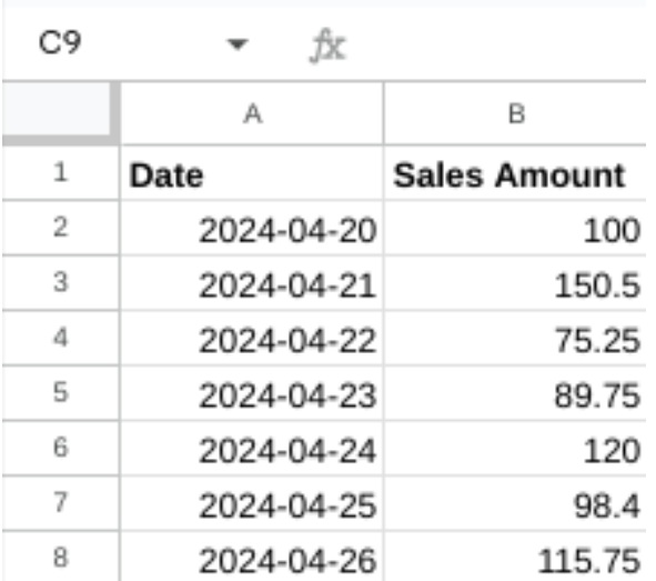
=SUMIFS(Sales_Amount_Range, WEEKNUM(Date_Range), Week_Number)

where

• Sales_Amount_Range: Points to the cells containing sales amounts (e.g., B2:B8)
• WEEKNUM(Date_Range): This extracts the week number from each date in the Date_Range (e.g., A2:A8). The WEEKNUM function converts dates to their corresponding week numbers.
• Week_Number: This is the specific week number for which you want to calculate the sum (e.g., enter 18 in a separate cell for the sum of week 18).

Result: By copying this formula down and changing the Week_Number in each cell, you'll get the total sales for each week.

Sum by month

You have a data table with information about monthly expenses, including columns for Date (date) and Expense Amount (number). You’re trying to find the total expenses for each month.

=SUMIFS(Expense_Amount_Range, MONTH(Date_Range), Month_Number)

where

• Expense_Amount_Range: points to the cells containing expense amounts (e.g., B2:B5)
• MONTH(Date_Range): This extracts the month number from each date in the Date_Range (e.g., A2:A5). The MONTH function isolates the month (1-12) from the date
• Month_Number: This is the specific month number you want to calculate the sum for (e.g., enter 3 in a separate cell for the sum of March expenses).

Result: Using this formula, you should get the total expenses for each month (e.g., March's total would be 209.00).

Sum of horizontal range

If you have a data table with sales figures for different products across various weeks (represented horizontally in the first row), you want to calculate the total sales for each product (vertically in a column).

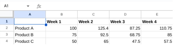
{=SUM(IF($A2:$D2=A2, $B2:$D2))} Entered with Ctrl+Shift+Enter or Command+Shift+Return

Where:

• $A2:$D2: week names (absolute row reference to fix when copied down)
• A2: product name we want the sum for (absolute column reference)
• $B2:$D2: sales figures for the product in A2 (absolute row reference)
• IF statement: Check if week names match the product name. If yes, include the corresponding sales figure.
• SUM(): sums the results from the IF statement (total sales for the product)

Result: The result of the formula =SUM(IF($A2:$D2=A2, $B2:$D2)) is the total sales for a specific product in a spreadsheet.

Sum of the month in columns

Here’s how to use SUMIFS function in Excel using two different methods.

1. MONTH & SUMIFS (Helper Column)

Step 1. Create a helper column (e.g., E) with =MONTH(A2:A10) (adjust ranges as needed) to extract month numbers from your date columns (A:D).

Step 2. Formula (assuming you want to sum columns B and C for April):

=SUMIFS(B2:B10, E2:E10, 4, C2:C10, E2:E10, 4) // 4 represents April

2. EOMONTH & SUMPRODUCT (Helper Columns)

Step 1. Create helper columns (e.g., E and F) with =EOMONTH(A2:A10,0) and =EOMONTH(B2:B10,0) (adjust ranges) to get the last day of the month for each date in columns A and B.

Step 2. Formula (assuming you want to sum column B for April using a date in A1):

=SUMPRODUCT((E2:E10 >= DATE(YEAR(A1), 4, 1)) * (F2:F10 <= DATE(YEAR(A1), 4, DAY(A1)))) * B2:B10) `

How to Look Up Excel SUMIFS With Multiple Criteria

Perform a SUMIFS function with multiple criteria in Excel with these steps:

• Select a cell where you want the result to appear.
• Type "=SUMIFS(" to start the function.
• Enter the range of cells containing the values you want to sum.
• Type "," to separate the arguments.
• Enter the first range of cells containing the criteria you want to apply.
• Type "," to separate the arguments.
• Enter the first criteria.
• Type "," to separate the arguments.
• Enter the second range of cells containing the second criteria.
• Type "," to separate the arguments.
• Enter the second criterion.
• Continue this pattern for additional criteria and ranges if needed.
• Close the function with ")" and press Enter.
  

Excel SUMIFS Wildcard

If you’re wondering how to use SUMIFS function in Excel with wildcards, here’s all you need to know.

Essentially, here are all the Excel SUMIFS wildcards that you can expect:

• Asterisk (*): A versatile card of its capacity, it will match any sequence of characters, even 0.

For instance, *Skirt* would find “Skirt”, “Short Skirt”, “Mid Skirt”, and so on.

• Question (?): This one matches any single character out there.

For *Pr?ce*, you could find “Price”, “Pruce”, “Place”. You name it.

Note that you need to use double quotes (“”) to receive SUMIFS results. The wildcards, by default, aren’t case-sensitive in SUMIFS.

Final Thoughts

To sum it up (quite literally), here is all that you need to know about how to use SUMIFS function in Excel. But if you’re a tad bit more curious, I would suggest checking out upGrad’s list of courses where you’d find the right platform to upscale faster. upGrad has a range of options you can choose from when it comes to the upskilling game. Check out our courses.

Get certified today!

Frequently Asked Questions

1. How do you use SUMIFS condition in Excel?

Here is how to use SUMIFS function in Excel: =SUMIFS(sum_range, criteria_range1, criteria1, [criteria_range2, criteria2], … With this formula, you will can sum all the values meeting the criteria.

2. How do you enter a SUMIF function?

To enter a SUMIF function, you enter =SUMIF and follow it up with an opening parenthesis. After this, you can specify the range, and criteria, along with the range to sum if the criteria are met.

3. How do I combine IF and SUMIFS in Excel?

If you want to combine IF and SUMIFS, you can nest the SUMIFS function within an IF function.

4. Can I use SUMIF for multiple criteria?

Although you cannot directly use SUMIF for multiple criteria, you can use the function for multiple criteria in Excel.

5. How do I add two conditions in SUMIFS?

If you want to add two conditions in SUMIFS, you have to specify the existing sum range with pairs of criteria range and criteria.

6. How do I sum multiple columns in SUMIFS?

To sum multiple columns in SUMIFS, use this formula: =SUMIFS(sum_range, criteria_range1, criteria1, criteria_range2, criteria2, criteria_range3, criteria3).

7. How do I sum 3 columns in Excel?

To sum 3 columns, specify three different criteria ranges and criteria pairs. Use this formula: =SUMIFS(A1:A10, D1:D10, criteria1, B1:B10, criteria2, C1:C10, criteria3). Replace the criteria with your conditions accordingly.

8. What is the array formula for SUMIFS?

SUMIFS does not require an array formula syntax as it can handle multiple criteria. You can directly use SUMIFS without using CTRL+Shift+Enter as you generally would with array formulas.

9. Does SUMIFS work on columns?

SUMIFS works perfectly fine with Excel columns. To do this, you can specify the criteria ranges and sum ranges covering the entirety of columns, specific ranges within columns, or even intersecting ranges within columns.