Central Limit Theorem

The central limit theorem is a very important concept in statistics used by statisticians all over the world. This theorem was first hinted at by Abraham de Moivre in 1733 and formalized by George Pólya in the 1920s. It states that when a big sample size is taken from a population with a finite variance, the sample means will form a normal distribution, which is regardless of the original distribution of the data.

This powerful theorem allows you to make predictions and conclude a population based on sample data, making it a cornerstone of statistical analysis. It is used in various fields from finance to engineering. Unpacking this complex definition can be challenging, but that is what this article is here to help with. I will explain the Central Limit Theorem thoroughly. We will discuss it with practical examples and look at its formulas, applications, and much more.

What is the Central Limit Theorem (CLT)?

The central limit theorem shows that given a sufficiently large sample size, the mean sampling distribution will always be regularly distributed. The sample distribution of the mean will be regular regardless of whether or not the population has a poisson, binomial, normal or any other distribution.

When you repeatedly take samples of a sufficiently large size (typically 30 or more) and calculate their means, these means will form a symmetrical, bell-shaped distribution known as a normal distribution. This holds true even if the data you are sampling from is not normally distributed.

For example, consider a population of people's shoe sizes, which might not follow a normal distribution. If you were to take multiple samples of 50 people's shoe sizes and calculate the mean for each sample, the distribution of those means would be roughly normal. 

The central limit theorem in statistics is immensely useful because it allows you to make inferences about the population mean using the normal distribution, simplifying analysis.

In mathematical terms, if a population has a mean (μ) and a standard deviation (σ), the distribution of the sample mean for a sample size (N) will have a mean (μ) and a standard deviation (σ/√N). As your sample size increases, the sample mean gets closer to the population mean.

Conditions of the Central Limit Theorem

For the Central Limit Theorem (CLT) to hold true, certain conditions must be met. These conditions ensure that the sampling distribution of the mean will approximate a normal distribution.

1. Sufficiently Large Sample Size

The sample size should be large enough, typically n≥30. This helps ensure that the distribution of the sample means will be normal.

2. Finite Variance

The population from which you are sampling should have a finite variance. The CLT does not apply to populations with infinite variance, such as the Cauchy distribution, though most real-world distributions do have finite variance.

3. Random Sampling

The samples must be drawn randomly from the population to ensure each sample has an equal chance of being selected.

4. Independent and Identically Distributed (i.i.d.) Samples

The samples need to be independent of each other and identically distributed. This means that the selection of one sample does not influence the selection of another, and each sample is drawn from the same population under the same conditions.

5. Sample Independence

Each sample should be independent, meaning the result of one sample does not affect the others.

6. Sample Proportion

When sampling without replacement, the sample size should not exceed 10% of the total population to maintain independence.

The Central Limit Theorem Formula

The Central Limit Theorem (CLT) is an amazing concept because it allows us to understand the shape of a sampling distribution without having to sample a population repeatedly. The parameters of the population determine the parameters of the sampling distribution of the mean. Here is how you can describe the sampling distribution:

• Mean of the Sampling Distribution: In this,  (X̄) is equal to the mean of the population (μ).
• Standard Deviation of the Sampling Distribution: Here, (σ/√n) is the population standard deviation (σ), which is divided by the square root of the given sample size (n).

This central limit theorem formula shows the distribution of the sample means X̄ will follow a normal distribution N with a mean μ and a standard deviation σ/√n.

Using this notation, you can summarize the sampling distribution of the mean or central limit theorem equation as follows:

Where:

• X̄ represents the distribution of the sample means.
• ∼ means "follows the distribution of."
• N denotes a normal distribution.
• μ is the mean of the population.
• The population standard deviation is represented by σ.
• n is the sample size.

Steps to Follow to Solve Problems with the Central Limit Theorem

When solving problems involving the Central Limit Theorem (CLT), especially those that involve inequalities such as >, <, or ranges (between two values), you can follow these steps to find the solution:

1. Identify the Problem Parameters

Determine the sample size (n), population mean (μ), and population standard deviation (σ). Also, identify the inequality or range given in the problem (e.g., >, <, or "between").

2. Draw a Graph with the Mean as the Center

Sketch a normal distribution curve, marking the population mean (μ) at the center. This visual aid helps you understand where the sample mean (X̄) falls within the distribution.

3. Calculate the Z-Score

Use the Z-score formula to standardize your sample mean. 

This step converts your sample mean to a Z-score, which you can use to find probabilities from the standard normal distribution.

4. Refer to the Z-Table

To determine the associated probability, check for the Z-score in the Z-table. The Z-table gives you the area under the standard curve to the left of the Z-score.

5. Adjust Based on Inequality

Types of adjusting based on inequality are explained below:

For problems involving >

Subtract the Z-table value from 1 to get the probability of the sample mean being greater than a certain value.

For problems involving <

Use the Z-table value directly to get the probability of the sample mean being less than a certain value.

For problems involving "between"

Calculate the Z-scores for both values and find their corresponding probabilities from the Z-table. Subtract the smaller Z-table value from the larger one to get the probability that the sample mean falls between the two values.

6. Convert the Probability

If needed, convert the decimal value obtained from the Z-table into a percentage by multiplying by 100.

An Example of the Central Limit Theorem 

Suppose you want to find the probability that the average height of a sample of 50 students is less than 5.8 feet, given that the population mean height is 5.6 feet, with a 0.5-feet standard deviation.

Identify parameters: n = 50, μ = 5.6, σ = 0.5, and the inequality X̄ < 5.8

Draw the graph with 5.6 at the center.

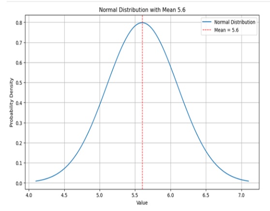
Calculate the Z-score:

Refer to the Z-table to find the probability corresponding to Z=2.83 (which is about 0.9977).

Since the problem involves <, use the Z-table value directly.

The probability is 0.9977, or 99.77%.

Applications of the Central Limit Theorem

As discussed, the Central Limit Theorem (CLT) is a powerful tool that helps you predict the characteristics of a population from a sample. Here are some practical uses of the CLT:

1. Economics and Data Science

Economists and data scientists use the CLT to determine a population, helping them build accurate statistical models.

2. Biology

The central limit theorem is used by biologists to help with research and experimentation by providing accurate predictions about population features based on sample data.

3. Manufacturing

In manufacturing, the CLT is used to estimate the proportion of defective items by analyzing random samples from production batches, ensuring quality control.

4. Surveys and Population Inferences

The CLT is essential in survey analysis, allowing you to predict population characteristics or average responses from sample surveys.

5. Machine Learning

The CLT helps in evaluating model performance and making inferences about data distributions, enhancing the development of robust machine learning models.

6. Finance

Investors use the CLT to analyze stock returns and construct diversified portfolios. For example, to analyze the return of a stock index with 1,000 equities, an investor might sample 30–50 stocks across various sectors to estimate the total index return, ensuring unbiased results.

7. Election Polls

An “application of the central limit theorem” is also in election polls. Pollsters use the CLT to estimate the percentage of people supporting a candidate, constructing confidence intervals to gauge public opinion accurately.

8. Income Analysis

CLT can also be used to calculate the mean family income in a country, providing insights into economic conditions and informing policy decisions.

9. Random Processes

The central limit theorem applies to rolling dice, flipping coins, and random walks, where the distribution of outcomes (like the total number of heads or distance covered) approaches a normal distribution as the number of trials increases.

10. More Central Limit Theorem Examples

Let's look at a few examples to better understand how the Central Limit Theorem (CLT) applies in different scenarios.

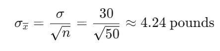
Example 1: Male Population's Weight

Imagine you are researching the weights of men in a certain population. The weight data follows a normal distribution with a mean (μ) of 180 pounds along with a standard deviation (σ) of 30 pounds. If you take a sample of 50 men, what would the mean and standard deviation of the sample be?

Solution:

Given: μ = 180 pounds, σ = 30 pounds, n = 50

According to the CLT, the sample mean is equal to the population mean.

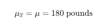
The sample mean's standard deviation is calculated as follows:

Example 2: General Distribution

Consider a distribution with a mean (μ) of 65 and a standard deviation (σ) of 300. If you draw a sample of 80 from this distribution, what would the mean and standard deviation of the sample be?

Solution:

Given: μ=65, σ=300, n=80

According to the CLT, the sample mean is equal to the population mean.

The sample mean's standard deviation is calculated as follows:

Final Thoughts

The Central Limit Theorem (CLT) is extremely important in statistical analysis. Based on the sample data, you can use it to make accurate predictions and come up with meaningful conclusions about a population. The above characteristics make it important for a range of fields that cut across economics, biology, manufacturing, and finance.

Through examples, we have seen how one can employ the central limit theorem to make sure that the distribution of sample means approximates normal distribution when the sample size is large enough. It can be said without fear of contradiction that grasping the central limit theorem and applying it will help simplify complex analysis and obtain valuable insights from any data set, regardless of its original nature.

FAQs

What is the Central Limit Theorem (CLT)?

The CLT states that the sampling distribution of the sample mean will approximate a normal distribution, given a sufficiently large sample size.

Why is the Central Limit Theorem important?

It enables users to infer population parameters using sample statistics, thereby making many statistical analyses simpler.

Does the Central Limit Theorem apply to all populations?

The CLT applies mostly to real-world populations where there is finite variance.

Why is the central limit theorem called central?

The Central Limit Theorem (CLT) is called central because it ensures that a sample mean forms a normal distribution, no matter the original population distribution.

What is the application of CLT?

In such areas as banking, manufacturing, medical science, or public opinion polls this CLT comes into play while predicting certain properties of total sets.

What are the advantages of CLT?

The CLT simplifies data analysis and enables accurate predictions and decisions based on sample data.

Are there any limitations to the Central Limit Theorem?

It requires a large sample size and only applies to populations with finite variance and independent, identically distributed samples.

Can any sample size be used to apply the Central Limit Theorem?

No, it generally requires a sample size of at least 30 to ensure a normal distribution of the sample mean.