Binomial Distribution

Introduction

Binomial distribution models the number of successes in a fixed number of independent trials with constant probability. The binomial distribution's roots trace back to the work of Swiss mathematician Jacob Bernoulli in the late 17th century. The concept has undergone subsequent improvements by Laplace, Pascal, and others.

The binomial distribution is fundamental in probability theory and statistics today. It is the cornerstone for modeling discrete random variables and precisely analyzing real-world phenomena. Here is a guide to the binomial distribution formula and its applications.

Binomial Distribution Definition 

The independent Bernoulli trials each contain the same probability of success. The section below covers the basic concepts of binomial distribution. 

Basic Concepts of Binomial Distribution 

1. Bernoulli Trials

Bernoulli trials are experiments or processes that have two possible outcomes. The outcomes of each trial can result in success or failure. Each trial is independent, and the result of one trial does not affect subsequent trials. A good example is flipping a coin (heads or tails) or rolling a die (success if a specific number comes up).

2. Trial Outcomes (Success and Failure)

Success typically represents the occurrence of an event of interest, while failure represents the event's non-occurrence. These outcomes are mutually exclusive, and only one of them can occur in a single trial.

3. Independence of Trials

Independence of trials means that the outcome of one trial does not influence the result of any other trial. Each trial is subject to the same conditions and probability of success or failure.

4. Probability of Success (p) and Failure (q)

You can use  'p' to denote the probability of success and 'q' to denote the probability of failure. The probabilities of success and failure must sum to (1: p + q = 1). The probability 'p' represents the likelihood of the desired outcome (success), while 'q' represents the likelihood of the alternative outcome (failure).

Binomial Distribution Function

The binomial distribution function is responsible for calculating the probability of obtaining a specific number of successes in a fixed number of independent Bernoulli trials with a constant success probability.

Binomial Distribution Formula

Below is a mathematical representation of the probability mass function (PMF). 

P(X-k) - (nk) * Pk * (1-p)n-k

Where: 

• P(X-k) is the probability of getting exactly 𝑘 successes in 𝑛 trials.
• (nk) is the binomial coefficient. It represents the number of ways to choose 𝑘 successes out of 𝑛 trials.
• (p) is the probability of success in a single trial.
• (1 - p) is the probability of failure in a single trial.
• k ranges from 0 to 𝑛 inclusive.
  

Binomial Distribution Probability Formula

The binomial distribution formula involves two main parameters and below is a summary. 

• n (number of trials): This parameter represents the total number of independent trials or experiments.
• p (probability of success): This parameter represents the probability of success for an individual trial. It is the probability of the event of interest occurring in a single trial.
  

Cumulative Distribution Function (CDF)

Below is the mathematical representation of the cumulative distribution function. 

Cumulative distribution function (CDF)

F(k)=P(X≤k)=∑i=0k​(in​)×pi×(1−p)n−i

Where:

• F(k) is the cumulative probability up to 𝑘.
• P(X ≤ k) represents the probability that the number of successes is less than or equal to 𝑘.
• (ni) is the binomial coefficient. It represents the number of ways to choose 𝑖 successes out of 𝑛 trials.
• k ranges from 0 to 𝑛, inclusive.

The CDF provides a way to assess the probability of achieving a certain number of successes or fewer in a binomial experiment. It is an essential method for analyzing the distribution of outcomes over a range of values.

Characteristics of the Binomial Distribution

The characteristics encompass fundamental properties, including probability distribution properties, mean and variance, skewness and kurtosis, and mode. Here is a highlight of the binomial distribution properties. 

Probability Distribution Properties

The binomial distribution exhibits several key probability distribution properties.

• Discreteness: The binomial distribution is a discrete probability distribution because it describes the probabilities of discrete outcomes (such as the number of successes in a fixed number of trials).
• Finite Support: The support of the binomial distribution is finite, ranging from 0 to 𝑛 inclusive, where 𝑛 is the number of trials in the experiment. 
• Non-Negative Probabilities: The probabilities assigned by the binomial distribution are non-negative, ensuring that the probability of observing any particular outcome is always greater than or equal to zero.
• Sum of Probabilities: The sum of probabilities for all possible outcomes equals 1.
  

Mean and Variance

The mean (μ) and variance (2) are important characteristics that describe the central tendency and spread of the distribution.

• Mean: You can calculate it as the product of the number of trials (𝑛) and the probability of success (𝑝): μ=n×p. The mean represents the average number of successes expected in 𝑛 trials.
• Variance (σ2): You can calculate it as the product of the number of trials (𝑛), the probability of success (𝑝), and the probability of failure: (1−𝑝): 𝜎2= 𝑛 × 𝑝 × (1−𝑝). The variance measures the spread or dispersion of the distribution around its mean. A larger variance indicates greater variability in the number of successes observed across trials.
  

Skewness and kurtosis

Skewness and kurtosis are two important characteristics that describe the shape of the distribution.

• Skewness: Measures the asymmetry of the probability distribution. Below is a mathematical representation of skewness in a binomial distribution. The magnitude of skewness decreases as 𝑛 increases, leading to a more symmetric distribution for large 𝑛.

• Kurtosis: Kurtosis measures the "tailedness" or the peakedness of the probability distribution. Below is a mathematical representation of kurtosis and excess kurtosis (kurtosis relative to a normal distribution). A binomial distribution with low 𝑛 can exhibit higher kurtosis, indicating a more peaked distribution with heavier tails. As 𝑛 increases, the kurtosis approaches that of a normal distribution, particularly when 𝑝 is not too close to 0 or 1.

Mode

The mode is the value(s) of the random variable 𝑋 that has the highest probability of occurring. You can calculate the mode by using the following mathematical equation. The ⌊x⌋ denotes the floor function, which rounds down 𝑥 to the nearest integer.

Mode = [(n + 1)p] or [(n+1)p] -1

If (𝑛+1) is an integer, then the binomial distribution has two modes: (𝑛+1)𝑝 and (n+1)p−1. If (𝑛+1) is not an integer, then the binomial distribution has a single mode a ⌊(𝑛+1)𝑝⌋.

Negative Binomial Distribution 

A negative binomial distribution is a discrete probability distribution that models the number of trials needed to achieve a specified number of successes in a sequence of independent and identically distributed Bernoulli trials. The mathematical formula below illustrates the probability mass function of a negative binomial distribution. 

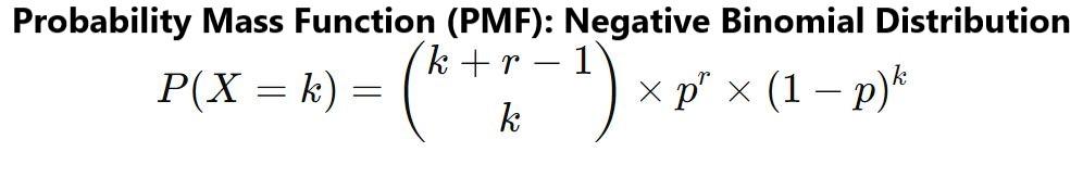
Where: 

• (k + r - 1k) is the binomial coefficient, representing the number of ways to arrange 𝑘 failures and 𝑟 successes in 𝑘+𝑟 trials.
• k is the number of failures, and 𝑋 represents the random variable for the number of failures before the 𝑟-th success.
  

Binomial Distribution Example 

Real-world applications for the binomial distribution are wide. Below is a summary of areas of application. 

• Coin Toss: Calculating the probability of getting a certain number of heads in multiple coin tosses.
• Quality Control: Determining the probability of finding a certain number of defective items in a batch.
• Survey Results: Estimating the number of people who will respond positively in a sample survey given a probability of a positive response.
• Clinical Trials: Evaluating the success rate of a new drug by comparing the number of patients who improve (success) to the number who do not (failure).
• Market Research: Determining the likelihood that a certain number of customers will prefer a new product over an existing one in a given sample size.
• Genetics: Calculating the probability of inheriting a specific trait based on Mendelian genetics.
• Epidemiology: Estimating the likelihood of a certain number of individuals contracting a disease in a population given an infection probability.
• Stock Market: Predicting the number of days a stock will close above a certain price in a month.
• Risk Management: Assessing the probability of defaults in a portfolio of loans.
  

Limitations and Assumptions

The binomial distribution has drawbacks because it relies on certain assumptions to work. The assumptions include a fixed number of trials (𝑛), two possible outcomes, constant probability of success (p), and independence of trials. The assumptions make the method unreliable in certain situations, as illustrated below.

• Variable Probability of Success: The binomial distribution is not suitable if the probability of success changes from trial to trial. 
• More Than Two Outcomes: The binomial distribution is inappropriate if each trial can result in more than two outcomes (e.g., dice rolling). 
• Dependent Trials: The binomial distribution does not apply if the trials are not independent. 
  

Alternatives for Non-Binomial Scenarios

Here are a couple of alternatives for non-binomial scenarios. 

Hypergeometric Distribution: Efficient method for sampling without replacement from a finite population.

Negative Binomial Distribution: You can use it to count the number of trials needed to achieve a fixed number of successes.

Multinomial Distribution: Generalizes the binomial distribution for scenarios with more than two possible outcomes for each trial.

Normal Distribution: Efficient when the number of trials is large, and both 𝑛𝑝 and (1−𝑝) are greater than 5, the normal distribution can approximate the binomial distribution (Central Limit Theorem).

Wrapping Up 

The binomial distribution has proven to be a crucial statistical tool for modeling or analyzing the probability of a fixed number of successes in a series of independent trials with constant success probability. You can see the use of binomial distribution in financial institutions, biology research centers, and quality control sectors. 

FAQs

1. What are the 4 properties of the binomial distribution?

Four properties of binomial distribution include a fixed number of trials, two possible outcomes, constant probability of success, and independence of trials. 

2. What is the full formula of binomial distribution?

The formula of the binomial distribution is P(X - k) - (nk) Pk(1-P)n-k.

3. What are the main features of binomial distribution?

The main features of the binomial distribution are discrete probability distribution, a fixed number of trials, two outcomes, and a constant probability of success. 

4. What are the types of binomial distribution?

The types of binomial distribution are symmetric, positively skewed, and negatively skewed. 

5. What is a binomial distribution with an example?

A binomial distribution models the number of successes in a fixed number of independent trials, like flipping a coin.

6. What is the use of binomial distribution?

The binomial distribution is an efficient method for predicting the number of successful outcomes in repeated trials with fixed probability.

7. What is the real-life application of binomial distribution?

The binomial distribution helps in fields like quality control to predict the number of defective items in a batch.