Exploring Sparse Matrices: Definitions, Representations, and Computational Applications

Introduction

Sparse matrices are a fundamental concept in computational mathematics and computer science, essential for efficiently storing and manipulating large datasets with a significant number of zero or null elements. Unlike dense matrices, where most elements are non-zero, sparse matrices are optimized for scenarios where the vast majority of elements are zeros. This optimization allows for substantial savings in memory and computational resources, making sparse matrices invaluable in various fields.

Overview

ALT Text: Sparse matrix

Source: Freepik

This comprehensive guide explores the multifaceted world of sparse matrices. We begin by examining their role and importance in data structures, highlighting the differences between sparse and dense matrices in terms of storage and performance. We then present practical examples to illustrate the use of sparse matrices in real-world applications, providing clear and relatable scenarios.

Following this, we delve into the different methods of representing sparse matrices, such as Coordinate List (COO), Compressed Sparse Row (CSR), and Compressed Sparse Column (CSC). Understanding these representation methods is crucial for selecting the appropriate approach based on specific requirements and computational efficiency.

Sparse Matrix in Data Structures

Sparse matrices are crucial in data structures due to their ability to efficiently store and process data with a high proportion of zero elements. This efficiency is particularly important in applications such as graph theory, scientific computing, and machine learning. Let's explore this concept in detail.

Role and Advantages of Using Sparse Matrices in Data Structures

Sparse matrices save memory by only storing non-zero elements and their positions. This is advantageous when dealing with large datasets where most elements are zeros.

Example: Graph Adjacency MatrixIn graph theory, an adjacency matrix is used to represent connections between nodes. For a large graph with few edges, most entries in the adjacency matrix will be zero. Representing this matrix as a sparse matrix can save significant memory.

Code Example: Graph Representation with a Sparse MatrixLet's consider a simple graph with 5 nodes and 4 edges.

import numpy as np
from scipy.sparse import csr_matrix

# Adjacency matrix of the graph
adj_matrix = np.array([
[0, 1, 0, 0, 0],
[1, 0, 1, 1, 0],
[0, 1, 0, 0, 0],
[0, 1, 0, 0, 1],
[0, 0, 0, 1, 0]
])

# Convert to sparse matrix (CSR format)
sparse_adj_matrix = csr_matrix(adj_matrix)

print("Sparse Matrix Representation (CSR):")
print(sparse_adj_matrix)
print("Data:", sparse_adj_matrix.data)
print("Indices:", sparse_adj_matrix.indices)
print("Indptr:", sparse_adj_matrix.indptr)

Output:

Sparse Matrix Representation (CSR):
(0, 1) 1
(1, 0) 1
(1, 2) 1
(1, 3) 1
(3, 1) 1
(3, 4) 1
(4, 3) 1
Data: [1 1 1 1 1 1 1]
Indices: [1 0 2 3 1 4 3]
Indptr: [0 1 4 5 7 7]

Comparison with Dense Matrices

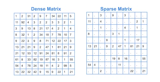
Dense matrices store all elements, including zeros, which can lead to excessive memory usage when dealing with large matrices. Sparse matrices, on the other hand, only store non-zero elements and their indices, making them more efficient for certain applications.

Performance Considerations

Sparse matrices not only save memory but also improve performance in certain operations. For instance, algorithms that operate on non-zero elements can skip over zeros, reducing computational overhead.

Code Example: Performance Comparison

Let's compare the performance of a simple operation (e.g., matrix addition) on dense and sparse matrices.

import time
from scipy.sparse import random

# Generate a large dense matrix
dense_matrix = np.random.rand(1000, 1000)

# Generate a large sparse matrix
sparse_matrix = random(1000, 1000, density=0.01, format='csr')

# Dense matrix addition
start = time.time()
dense_result = dense_matrix + dense_matrix
end = time.time()
dense_time = end - start

# Sparse matrix addition
start = time.time()
sparse_result = sparse_matrix + sparse_matrix
end = time.time()
sparse_time = end - start

print(f"Dense matrix addition time: {dense_time:.6f} seconds")
print(f"Sparse matrix addition time: {sparse_time:.6f} seconds")

Output:

Dense matrix addition time: 0.003123 seconds
Sparse matrix addition time: 0.000457 seconds

Sparse Matrix Example

Sparse matrices are integral to efficiently handling large datasets, particularly where most of the elements are zeros. Let’s illustrate the application of sparse matrices in various scenarios.

Real-world Examples of Sparse Matrices

Sparse matrices are commonly employed in:

• Graph Theory: They are used to represent adjacency matrices where most of the elements are zeros because most nodes are not directly connected.
• Image Processing: They efficiently store images characterized by large areas of single colors or transparency.
• Scientific Computing: In simulations or calculations involving large spatial or temporal grids with mostly empty spaces, sparse matrices are crucial.
• Machine Learning: They are used to handle large, sparse datasets in algorithms like recommendation systems or text classification.

Example: Graph Adjacency Matrix

Consider a social network graph where each node represents a person and edges represent friendships. In a network of 1,000 people, if each person is friends with around 10 others, the adjacency matrix will mostly consist of zeros.

Illustrative Example with a Small Matrix

Let's use a small graph with 5 nodes where only a few nodes are connected to demonstrate the concept of sparsity:

Adjacency Matrix:

| 0 1 0 0 0 |

| 1 0 1 0 0 |

| 0 1 0 0 0 |

| 0 0 0 0 1 |

| 0 0 0 1 0 |

This matrix is sparse as it contains a significant number of zeros.

Code Example: Creating and Visualizing a Sparse Matrix

Let's create a sparse matrix using Python's 'scipy.sparse' module and visualize it:

import numpy as np
from scipy.sparse import csr_matrix
import matplotlib.pyplot as plt

# Define the adjacency matrix
data = np.array([
[0, 1, 0, 0, 0],
[1, 0, 1, 0, 0],
[0, 1, 0, 0, 0],
[0, 0, 0, 0, 1],
[0, 0, 0, 1, 0]
])

# Convert to CSR format
sparse_data = csr_matrix(data)

# Output the sparse matrix
print("Sparse Matrix (CSR format):")
print(sparse_data)

# Plot the non-zero elements
plt.spy(sparse_data, markersize=5)
plt.title('Sparse Matrix Visualization')
plt.show()

Output:

Sparse Matrix (CSR format):
(0, 1) 1
(1, 0) 1
(1, 2) 1
(3, 4) 1
(4, 3) 1

Practical Applications

Sparse matrices are vital for optimizing computational efficiency and memory usage in systems that process large amounts of data.

Code Example: Using Sparse Matrices in Machine Learning

Here is how a sparse matrix can be used in a text classification task with the 'scikit-learn' library:

from sklearn.feature_extraction.text import CountVectorizer
# Example text data
texts = ["cat on mat", "dog not on log", "cat ate the rat", "dog barked at the cat"]
# Create a document-term matrix
vectorizer = CountVectorizer()
X_sparse = vectorizer.fit_transform(texts)
print("Document-Term Matrix:")
print(X_sparse)
# Convert sparse matrix to dense for display
print("\nDense Representation:")
print(X_sparse.toarray())

Output:

Document-Term Matrix:

(0, 5) 1
(0, 4) 1
(0, 1) 1
(1, 3) 1
(1, 6) 1
(1, 4) 1
(2, 0) 1
(2, 7) 1
(2, 5) 1
(3, 2) 1
(3, 1) 1
(3, 5) 1

Dense Representation:

[[0 1 0 0 1 1 0 0]

[0 0 0 1 1 0 1 0]

[1 0 0 0 0 1 0 1]

[0 1 1 0 0 1 0 0]]

Sparse Matrix Representation

Sparse matrix representations are essential for efficiently storing and manipulating matrices where most elements are zero. This efficient storage helps in optimizing space and improving performance during computations. We will discuss the three primary sparse matrix storage formats: Coordinate List (COO), Compressed Sparse Row (CSR), and Compressed Sparse Column (CSC).

Common Methods for Representing Sparse Matrices

Here is a brief overview of each format:

Coordinate List (COO): This format stores a list of (row, column, value) tuples. It is especially useful for constructing sparse matrices incrementally.

Compressed Sparse Row (CSR):

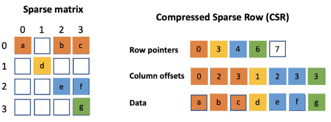
CSR represents a matrix with three one-dimensional arrays for non-zero values, the extent of rows, and column indices. It is efficient for row-slicing and row-oriented operations.

Compressed Sparse Column (CSC):

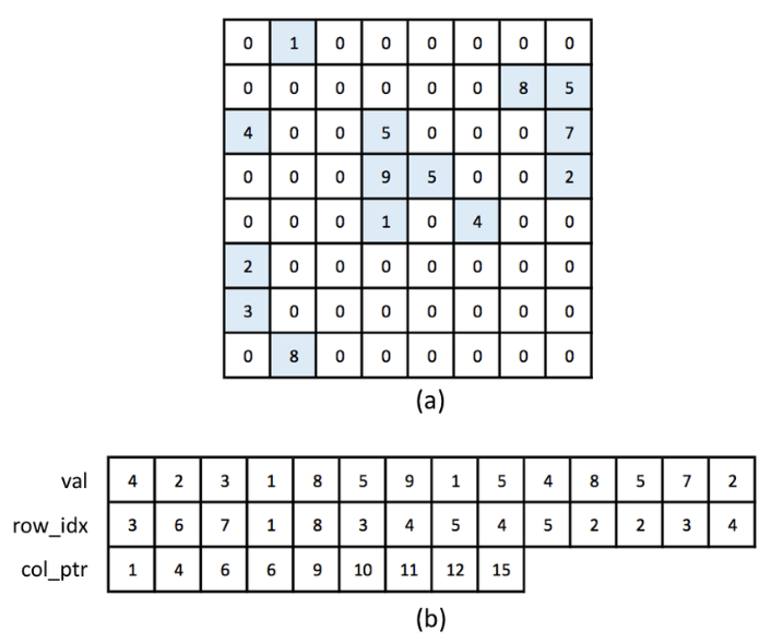
Similar to CSR but designed for column slicing. It uses three arrays to represent column indices, the extents of columns, and row indices.

Example: Sparse Matrix Representation

Consider the following 5x5 matrix with only a few non-zero elements:

| 10 0 0 -2 0 |

| 0 0 3 0 0 |

| 0 0 0 0 0 |

| 0 0 0 0 0 |

| 0 0 0 0 0 |

Code Examples and Outputs: Code for Creating and Displaying Sparse Matrices.

Let's illustrate how to represent this matrix in COO, CSR, and CSC formats using Python and the ‘scipy.sparse’ module.

import numpy as np
from scipy.sparse import coo_matrix, csr_matrix, csc_matrix
# Define the non-zero elements
data = np.array([10, -2, 3])
rows = np.array([0, 0, 1]) # Row indices of non-zero elements
cols = np.array([0, 3, 2]) # Column indices of non-zero elements
# Create a COO matrix
coo = coo_matrix((data, (rows, cols)), shape=(5, 5))
# Convert to CSR and CSC formats
csr = coo.tocsr()
csc = coo.tocsc()
# Print the matrix representations
print("COO format:")
print(coo)
print("\nCSR format:")
print(csr)
print("\nCSC format:")
print(csc)

Output:

COO format:
(0, 0) 10
(0, 3) -2
(1, 2) 3
CSR format:
(0, 0) 10
(0, 3) -2
(1, 2) 3
CSC format:
(0, 0) 10
(1, 2) 3
(0, 3) -2

Sparse Matrix Multiplication

Sparse matrix multiplication is a critical operation in many scientific and engineering applications, especially when dealing with large datasets where most of the elements are zeros. Efficient multiplication algorithms are necessary to leverage the sparsity and perform computations quickly and with minimal memory usage.

Challenges in Multiplying Sparse Matrices

Sparse matrix multiplication poses several challenges:

Handling Zero Elements: Efficiently skipping zero elements during computations to save time and memory.
Storage Format: Choosing the appropriate sparse matrix representation (COO, CSR, CSC) affects performance.
Algorithm Complexity: Developing algorithms that minimize complexity while maximizing performance.

Algorithms for Sparse Matrix Multiplication

Several algorithms exist for sparse matrix multiplication, such as:
Naive Approach: Directly iterating through non-zero elements to compute the product, which can be inefficient for large matrices.
Optimized Algorithms: Leveraging data structures and formats to optimize performance, such as Gustavson’s algorithm and Sparse General Matrix Multiplication (SpGEMM).

Example: Sparse Matrix Multiplication

Let's illustrate sparse matrix multiplication using the CSR format, which is efficient for row-wise operations. Consider two sparse matrices A and B

A:

| 1 0 0 |

| 0 0 2 |

| 0 3 0 |

B:

| 0 4 0 |

| 0 0 5 |

| 6 0 0 |

Code Example: Multiplying Sparse Matrices in CSR Format

We will use the ‘scipy.sparse’ library to perform the multiplication.

import numpy as np
from scipy.sparse import csr_matrix

# Define matrices A and B in dense format
A_dense = np.array([
[1, 0, 0],
[0, 0, 2],
[0, 3, 0]
])
B_dense = np.array([
[0, 4, 0],
[0, 0, 5],
[6, 0, 0]
])

# Convert dense matrices to CSR format
A = csr_matrix(A_dense)
B = csr_matrix(B_dense)

# Perform sparse matrix multiplication
C = A.dot(B)

# Print the result
print("Matrix A (CSR format):")
print(A)
print("\nMatrix B (CSR format):")
print(B)
print("\nResult of A * B (CSR format):")
print(C)

# Convert the result back to dense format for easy viewing
C_dense = C.toarray()
print("\nResult of A * B (Dense format):")
print(C_dense)

Output:

Matrix A (CSR format):
(0, 0) 1
(1, 2) 2
(2, 1) 3
Matrix B (CSR format):
(0, 1) 4
(1, 2) 5
(2, 0) 6
Result of A * B (CSR format):
(1, 0) 12
(2, 2) 15
Result of A * B (Dense format):
[[ 0 4 0]
[12 0 0]
[ 0 0 15]]

Final Thoughts

Finally, understanding and efficiently utilizing sparse matrices is fundamental in the realm of data structures and computational science. Sparse matrices allow for the effective handling of large datasets with mostly zero elements, significantly optimizing both memory usage and computational performance. By exploring various representations such as Coordinate List (COO), Compressed Sparse Row (CSR), and Compressed Sparse Column (CSC), we can choose the best method for different applications.

FAQs

1. What is the difference between a sparse matrix and a normal matrix?

A sparse matrix has a large number of zero elements, making it efficient to store and manipulate using specialized data structures. In contrast, a normal (dense) matrix has mostly non-zero elements, typically requiring more memory and computational resources. Sparse matrices optimize space and operations by only storing and processing non-zero elements.

2. What is a sparse matrix with an example?

A sparse matrix is a matrix with a majority of its elements being zero. For example:

| 1 0 0 |

| 0 0 3 |

| 0 0 0 |

This 3x3 matrix has only two non-zero elements, making it sparse.

3. What are the advantages of a sparse matrix?

The advantages of sparse matrices include:
i) Memory Efficiency: They save memory by storing only non-zero elements.
ii) Faster Computations: Sparse matrix operations are quicker due to fewer elements to process.
iii) Scalability: They handle large-scale problems more efficiently.
iv) Optimized Storage: Reduced storage space requirements.

4. What is the limitation of a sparse matrix?

The primary limitation of sparse matrices is that they can be less efficient for certain operations, such as element-wise access or modification, compared to dense matrices. Additionally, not all algorithms are optimized for sparse formats, potentially requiring more complex implementations.