Splay Trees: A Self-Adjusting Data Structure

Introduction

Imagine a library in which the most popular books are constantly at your fingertips. No greater long searches through dusty shelves—the librarians anticipate your wishes and keep your favorite with ease available. This is the essence of a splay tree, a self-adjusting records shape that prioritizes often accessed elements.

Built on Binary Search Trees

Splay tree timber is a type of binary seek tree (BST). In a BST, each node has a value, and all values within the left subtree are smaller, while all values inside the right subtree are large. This structure allows for efficient looking, insertion, and deletion with a time difficulty of O(log n) within the average case.

However, BSTs can turn out to be unbalanced if the insertion pattern is skewed. In this approach, a few searches may require traversing an extended route, negating the efficiency benefit.

Operations in a Splay Tree

Operations in a splay tree are explained below:

• Splay Tree Insertion: To insert a new element into the tree, start by performing a normal binary search tree insertion. Then, observe rotations to convey the newly inserted detail to the root of the tree.
• Splay Tree Deletion: To delete an element from the tree, first find the usage of a binary seek tree search. Then, if the element has no kids, absolutely take it away. If it has one child, promote that child to its function in the tree. If it has youngsters, discover the successor of the element (the smallest detail in its proper subtree), change its key with the element to be deleted, and delete the successor as a substitute.
• Splay Tree Search: To look for an element within the tree, begin by acting as a binary search tree seek. If the element is located, observe rotations to deliver it to the root of the tree. If it is not located, observe rotations to the ultimate node visited in the seek, which turns into the new root.
• Splay Tree Rotation: The rotations used in a splay tree are either a Zig or a Zig-Zig rotation. A Zig rotation is used to carry a node to the foundation, while a Zig-Zig rotation is used to stabilize the tree after more than one access to factors in the same subtree.
  

What is a Splay Tree in Data Structure?

When you use BSTs (Binary Search trees) for searching the information, the time complexity in the mean case is O(log2N). This is because the average case top of a binary tree is O(log2N). However, the worst case may be a left or proper-skewed tree, i.e., a linear tree. In such case the worst-case time complexity of the operations like looking, insertion, and deletion becomes O(N).

However, what if the timbers are made self-balancing such that they are by no means shape-skewed structures and the height constantly remains O(log2N)? This is completed with AVL timber and red-black bushes. These are self-balancing BSTs; therefore, the worst-case time difficulty of searching, insertion, and deletion is O(log2N).

However, the query is, are we able to do more than this? The solution is sure. In a few realistic scenarios, we can do better than AVL and red-black trees. How? Using splay timber.

The essential concept of splay timber is based on the “maximum often used factors”. A splay tree in data structure entails all of the operations of an everyday binary search tree, i.e., looking, insertion, deletion, etc. However, it is also one special operation, i.e., usually completed and it is often referred to as splaying.

The concept is to carry the more often used factors towards the basis of the BST so that if they are searched once more, they may be determined extra fast as compared to the less frequently used factors.

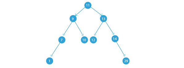
Consider the BST proven below.

Let’s say we want to search for 8. So, we start from the basis node. Since the price at the foundation node is 10 and we are looking for 8, i.e., a smaller element than the current node, we can circulate towards the left.

So, we visited the next node and we discovered eight. This is an everyday search operation in BST. However, we can do a little greater than this within the splay tree. We will carry out splaying, i.e., eight will now emerge as the foundation node of the tree.

How? We can try this with Some Rotations

There are six exceptional kinds of splay tree rotations. These include:

1. Zig Rotation or Right Rotation

2. Zig Zig Rotation or 2 Zig Rotations or 2 right rotations

3. Zag Rotation or Left Rotation

4. Zag Zag Rotation 2 Zag rotations or 2 left rotations)

5. Zig Zag Rotation (Right-Left Rotation, i.e., First do Zig, then Zag)

6. Zag-Zig Rotation (Left-Right Rotation, i.e., First do Zag, then Zig)

Let us have a look at those rotations one by one.

Zig Rotation or Right Rotation

Consider the tree proven underneath.

.

Source: Amazonaws.com

In this rotation, we circulate each node to 1 role in the direction of its proper. This rotation is used when the element that we are looking for is both a gift in the root node of the BST or a gift within the left infant of the foundation node.

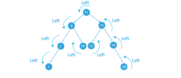
Suppose we are searching for node 9. This approach means that we are searching for the left child of the foundation node. So, we will carry out the zigzag rotation.

So, the steps for looking at node 9 are the same as when we perform the search in BST, and features have already been mentioned. Now, since that is the zig-zag rotation, i.e., we want to rotate every element 1 function to its right. This rotation is proven underneath.

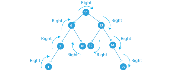
Alt Text: Zig rotation or right rotation

Source: Amazonaws.com

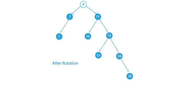
So, every element has to move from 1 position to its proper. Now, we will believe every detail going to at least one function to its right, and we believe that nine will become the root node, 11 will be its right child, and the left baby will be 7. What about node 10?

So, node 10 is the proper baby of node 9 earlier than rotation. So, after rotation, it is going to stay in the right subtree of node nine. However, it will now emerge as the left toddler of node eleven, as proven below.

Source: Amazonaws.com

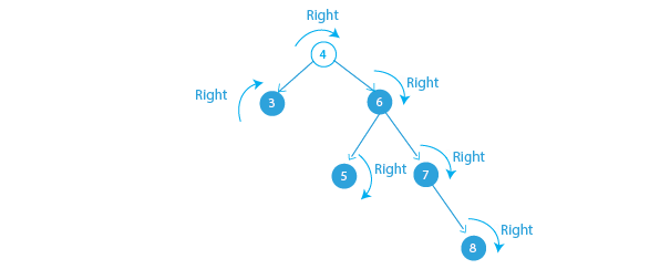
Zig-Zig Rotation or Right-Right Rotation

In this rotation, 2 proper rotations are achieved, one after another. The desired element is not the root node or the left child of the root node. Instead, it is located below the left subtree of the parent node. This means that the node has both a parent and a grandparent. Consider the tree shown beneath.

Source: Amazonaws.com

So, if we are trying to find node 3, we discover it at the final degree. Now, we can perform the first proper rotation.

Zig-Zig Rotation or Right-Right Rotation

After one rotation, the tree is displayed below. We perform the next rotation.

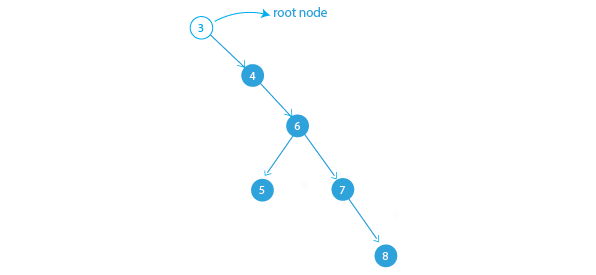
So, after 2 right rotations, node 3 is now the root node.

Zag Rotation or Left Rotation

Again, consider the tree shown below.

The Zag rotation, or the left rotation, is finished, while the element that we are searching for is both the root node and the right toddler of the root node.

So, take into account that we are attempting to find node thirteen. Since it is miles the right child of the root node, we carry out the zigzag rotation. Every element will rotate and attain 1 role in the present day. This is proven below.

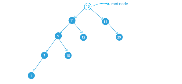
So, on account of the fact that after rotation, 14 has to end up being the right baby of 13, and 12 has to be changed into a gift as its left toddler, 12 will remain in the left subtree but will become the proper child of node 11. Node 13 has ended up being the root node now.

ZIg-Zag Rotation or Left-Left Rotation

The sequence of zig rotations might be followed by a series of zag rotations. The zig-zag rotation is used while the figure node and the grandparent node of a node are in LR or RL courting with each other. Consider the tree shown underneath.

Zag- Zag Rotation or Left-Left Rotation

Here, we perform 2 left rotations. Again, it is done when looking for an element (not the root or the right child of the root) but it should be present in the right subtree. It has both parents and grandparents. So, look at the tree shown below.

If we are searching 7, the result of the zag-zag rotation is shown below.

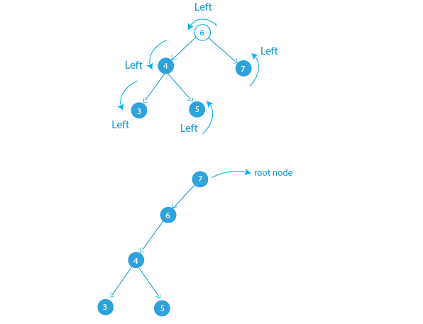
So, node 7 is now the root node of the tree.

Zig Zag Rotation or Right Left Rotation

This is a sequence of zig rotations, followed by a sequence of zag rotations. It is used is used when the parent node and the grandparent node are in an LR or RL relationship with each other. Consider the tree shown below.

Still, the parent and grandparent are in an RL relationship with each other if we want to search 5. Hence, we start with the Right rotation. Zig rotation about node 6, and the left rotation i.e. Zag rotation about the root node i.e. node 4. This completes the Zig Zag rotation. This is shown below.

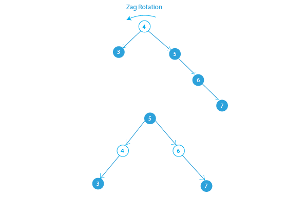
Eventually, we can see that 5 is the root node. So, this is Zig Zag rotation.

Zag-Zig Rotation or Left-Right Rotation

It is similar to the zig-zag rotation but the only difference is that first the left rotation happens and then the right one. Consider the tree proven below.

.

So, if we want to search 5, the rotation is shown below.

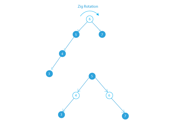
So, we can see that node five is at the foundation of the tree. This is Zag Zig Rotation.

Now that we have studied the splay timber, allow us to put into effect those rotations and other operations of a splay tree in data structure with an example of splay tree visualization shown underneath.

• C++
• Java
• Python

#include <bits/stdc++.h>
usingnamespace std;
class node
{
public:
int key;
node *left, *right;
};
node *TreeNode(int key)
{
node *Node = newnode();
Node->key = key;
Node->left = Node->right = NULL;
return(Node);
}
node *rightRotate(node *x)
{
node *y = x->left;
x->left = y->right;
y->right = x;
return y;
}
node *leftRotate(node *x)
{
node *y = x->right;
x->right = y->left;
y->left = x;
return y;
}
node *splay(node *root, int key)
{
if(root == NULL || root->key == key)
return root;
if(root->key > key)
{
if(root->left == NULL)
return root;
// Zig-Zig Rotation
if(root->left->key > key)
{
root->left->left = splay(root->left->left, key);
root = rightRotate(root);
}
elseif(root->left->key < key)// Zig-Zag
{
root->left->right = splay(root->left->right, key);
if(root->left->right != NULL)
root->left = leftRotate(root->left);
}
return(root->left == NULL) ? root : rightRotate(root);
}
else
{
if(root->right == NULL)
return root;
// Zag-Zig Rotation
if(root->right->key > key)
{
root->right->left = splay(root->right->left, key);
if(root->right->left != NULL)
root->right = rightRotate(root->right);
}
elseif(root->right->key < key)
{
root->right->right = splay(root->right->right, key);
root = leftRotate(root);
}
return(root->right == NULL) ? root : leftRotate(root);
}
}
node *bstSearch(node *root, int key)
{
returnsplay(root, key);
}
voidpreOrder(node *root)
{
if(root != NULL)
{
cout<< root->key <<" ";
preOrder(root->left);
preOrder(root->right);
}
}
intmain()
{
node *root = TreeNode(100);
root->left = TreeNode(50);
root->right = TreeNode(200);
root->left->left = TreeNode(40);
root->left->left->left = TreeNode(30);
root->left->left->left->left = TreeNode(20);
root = bstSearch(root, 20);
preOrder(root);
return 0;
}

Final Thoughts

So, we have pointed out the splay tree in statistics and its various rotation operations in a splay tree, as well as its time complexity. We desire that you favor the discussion and understand the idea.

FAQs

1. What is the difference between a BST and a splay tree?

• BST: Not assured balanced, common O(log n) access, can degrade to O(n) worst-case.
• Splay Tree: Self-balancing via splaying, O(log n) amortized access for all operations.

2. What are splay trees good for?

Dynamic statistics units with unpredictable get-right of entry to styles (cache management, community routing, etc.).

3. How does a splay tree differ from an AVL tree?

• AVL Tree: Strictly enforces height difference for stability (extra complex rebalancing).
• Splay Tree: Splaying promotes accessed factors to root for balance (easier but more frequent rebalancing).

4. Can you give an example of a splay?

Imagine attempting to find an element in a splay tree. Splaying brings that detail in the direction of the foundation for faster entry into destiny.

5. Is a splay tree self-balancing?

Yes, splaying continues stability via selling accessed factors to the foundation.

6. What is the cons of using splay trees?

• More complicated implementation compared to BSTs.
• Constant rebalancing can be highly-priced for very common operations.

7. Is there another name for a splay tree?

No, splay trees are not usually regarded by other names.

8. What is the runtime of splay trees?

O(log n) amortized for search, insertion, and deletion.

9. What is the minimum height of a splay tree?

1 (single node) or 2 (root and infant). It depends on getting entry to patterns, however splaying normally maintains it logarithmic.