Introduction
Bipartite Graph is one of the most fundamental structures in graph theory. It divides vertices into two disjoint sets where each edge links nodes from different sets. This simple idea makes bipartite graphs powerful tools in computer science, scheduling, matching problems, and network theory.
A special type, the Complete Bipartite Graph, connects every vertex in one set to every vertex in the other. Understanding these graphs helps you solve practical problems and build efficient algorithms. In this tutorial, we’ll cover definitions, properties, applications, and their role in real-world problem-solving. So, let’s start by understanding the bipartite graph.
Boost your tech skills with our Software Engineering courses and take your expertise to new heights with hands-on learning and practical projects.
What is a bipartite graph?
A bipartite graph is a particular type of graph within the broader study of graph theory. Their defining characteristic is that they can be partitioned into two sets such that no two vertices within the same set are adjacent to each other.
- Definition and Theory: bipartite graphs, as the name suggests, can be split into two parts. These parts are made in such a way that every edge of the graph connects a vertex in the first part to a vertex in the second part.
- Bipartite graph Properties: Some properties of bipartite graphs include that they don't contain odd length cycles and all their cycles have an even number of edges.
- Bipartite graph definition with example: Consider the following example: There are two sets of vertices {a, b, c} and {1, 2, 3}. Edges are a-1, b-2, and c-3.
- Key Applications: Applications include modeling relationships between different types of objects (like users and groups in social networks), matching problems, and network flows.
Take your programming skills to the next level and gain expertise for a thriving tech career. Discover top upGrad programs to master data structures, algorithms, and advanced software development.
Complete Graph
A complete graph is a type of graph in which every pair of distinct vertices is connected by a unique edge. In other words, it's a graph where every vertex is directly connected to every other vertex. In the case of a Complete bipartite graph, each node from one set forms a connection with all the nodes of the other set.
Complete graphs are denoted as Kn, where "n" represents the number of vertices.
Here is an example of a complete graph with 4 vertices (A, B, C, and D):
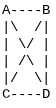
In this graph, each vertex is directly connected to every other vertex with a unique edge. For 4 vertices, there are a total of 6 edges. Complete graphs are commonly used in graph theory to illustrate concepts and algorithms due to their simplicity and symmetry.
Regular Graph
A regular graph is a graph where all vertices have the same degree, meaning they are connected to the same number of edges. In a regular graph, each vertex has an identical number of adjacent vertices. Regular graphs are often denoted as "k-regular," where "k" is the degree of each vertex.
Here's an example of a 3-regular graph with 4 vertices (A, B, C, and D):
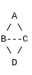
In this graph, each vertex is connected to exactly 3 other vertices, resulting in a regular graph. Regular graphs can have various degrees, and they often represent structured relationships in real-world scenarios.
Euler Path
An Euler Path is a path in a graph that visits every edge exactly once. This means that you start at a vertex, traverse edges to other vertices, and eventually end at a different vertex, covering every edge in the graph without repetition. If you can find an Euler Path in a graph, it suggests a specific sequence in which you can traverse the edges.
However, not all graphs have Euler Paths. There are specific conditions that must be met:
- Eulerian Circuit: If the Euler Path starts and ends at the same vertex, it's called an Eulerian Circuit. Not all graphs have Eulerian Circuits either.
- Vertex Degrees: In a connected graph, an Euler Path or Eulerian Circuit is possible if and only if there are either 0 or 2 vertices with an odd degree (number of edges incident to the vertex).
For example, let's consider a graph where two vertices have odd degrees (C and E):
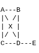
In this graph, vertices C and E have an odd degree. This means that an Euler Path or Circuit is not possible. The condition of having either 0 or 2 vertices with odd degrees is violated.
On the other hand, if we modify the graph slightly to ensure there are exactly 2 vertices with odd degrees:

In this case, vertices C and E have an odd degree, which satisfies the condition. An Euler Path (not a circuit) is possible in this graph, where you start at A, traverse all edges, and end at E.
State and Prove Euler's Theorem
Euler's Theorem states that a graph G has an Euler circuit if and only if every vertex of G has even degree. The theorem holds true for bipartite graphs, as the number of edges incident with a vertex determines whether the vertex's degree is even or odd.
Euler's Theorem Component | Description |
Theorem Statement | A graph G possesses an Euler circuit if and only if every vertex of G has even degree. |
Meaning | A graph has a path that traverses every edge exactly once and returns to its starting point, if and only if each of its vertices is connected to an even number of other vertices. |
Relation with bipartite graphs | The theorem applies to bipartite graphs as the degrees of vertices determine whether an Euler circuit exists. |
Proof Method | The theorem is proved using methods of induction and graph traversal. The proof focuses on the existence of a closed circuit in a graph with vertices of even degree. |
Bipartite Graph Algorithm
There are several algorithms and techniques to determine if a given graph is bipartite. One common algorithm is the Breadth-First Search (BFS) algorithm.
Here's a step-by-step explanation of how the BFS algorithm can be used to determine if a graph is bipartite:
- Choose a Starting Vertex: Start by selecting an arbitrary vertex from the graph as the starting point.
- Initialize Vertex Sets: Create two sets, often called "Set A" and "Set B," to store the two disjoint sets of vertices.
- Initialize Color Map: Assign colors (often represented as 0 and 1) to the starting vertex. Place the starting vertex in Set A.
- Queue Initialization: Enqueue the starting vertex into a queue for BFS traversal.
- BFS Traversal:
- While the queue is not empty:
- Dequeue a vertex from the queue.
- Traverse all neighboring vertices of the dequeued vertex.
- If a neighboring vertex doesn't have a color assigned:
- Assign the opposite color to the neighboring vertex and place it in the respective set.
- Enqueue the neighboring vertex into the queue.
- If a neighboring vertex has the same color as the current vertex, the graph is not bipartite.
- Repeat BFS: Repeat steps 4 and 5 until all vertices have been visited or until a conflict is detected.
Result: If no conflicts arise during BFS traversal (i.e., all edges connect vertices of different colors), the graph is bipartite. If there's a conflict, the graph is not bipartite.
Pseudocode for Bipartite Graph Detection using BFS:
function isBipartite(graph, start_vertex):
    create sets SetA and SetB
    create a color map for vertices

    assign color 0 to start_vertex
    add start_vertex to SetA

    create a queue and enqueue start_vertex

    while queue is not empty:
        current_vertex = dequeue from queue

        for each neighbor in graph[current_vertex]:
            if neighbor is not colored:
                assign opposite color to neighbor
                add neighbor to the respective set
                enqueue neighbor into the queue
            else if neighbor has the same color as current_vertex:
                return "Not Bipartite"
    return "Bipartite"

Call isBipartite(graph, any_starting_vertex)
We must also remember that this algorithm assumes the graph is connected. If the graph consists of multiple components, you should apply the BFS algorithm on each component. This algorithm works well for both directed and undirected graphs and is a common approach to determine whether a graph is bipartite or not.
Another method to determine if a graph is bipartite is to use graph coloring with the concept of two-coloring. This method doesn't necessarily require BFS traversal.
Here's how bipartite graph detection works using graph coloring:
- Choose a Starting Vertex: Start by selecting an arbitrary vertex from the graph.
- Initialize Vertex Colors: Assign colors (often represented as 0 and 1) to the starting vertex. This vertex will be part of Set A.
- Color Propagation:
- Traverse through the graph's vertices.
- For each vertex, if it's not colored:
- Assign the opposite color to the vertex.
- Traverse all neighboring vertices and assign the opposite color to them as well.
- Continue this process until all vertices are colored or until a conflict is detected.
- Conflict Detection: If you encounter a vertex that has a neighbor with the same color, the graph is not bipartite.
Result: If no conflicts arise (i.e., all edges connect vertices of different colors), the graph is bipartite.
Pseudocode for Bipartite Graph Detection using Graph Coloring:
function isBipartite(graph, start_vertex):
    create a color map for vertices

    assign color 0 to start_vertex

    for each vertex in graph:
        if vertex is not colored:
            assign opposite color to vertex

            for each neighbor in graph[vertex]:
                assign opposite color to neighbor
                if neighbor has the same color as vertex:
                    return "Not Bipartite"
    return "Bipartite"

Call isBipartite(graph, any_starting_vertex)
This method directly assigns colors to vertices based on their adjacency relationships, without explicitly performing BFS traversal. If you don't encounter a conflict during the color propagation process, the graph is bipartite.
Read these: Top Trending Tutorials of Python
Conclusion
We have explored the concept of the Bipartite Graph, covering its definition, properties, examples, and related ideas. Gaining a clear understanding of bipartite graphs strengthens your foundation in graph theory and sharpens your problem-solving skills. These concepts are widely applied in computer science, data science, and network design, making them valuable for academic growth and professional careers.
To build deeper expertise and apply concepts like Bipartite Graph and Complete Bipartite Graph to real-world problems, upGrad offers structured courses guided by industry experts, helping you stay ahead in competitive fields
FAQs
1. What is the example of Bipartite Graph?
Consider a graph with two sets of vertices: {a, b, c} and {1, 2, 3}. Edges exist as a-1, b-2, and c-3. This forms a Bipartite Graph because all edges connect vertices from different sets, with no intra-set connections. Such examples demonstrate the basic structure and two-set division used in many applications like user-item mapping.
2. How is a Bipartite Graph different from a Complete Graph?
In a Complete Graph, every vertex connects to every other vertex. In a Complete Bipartite Graph, each vertex in one set connects to all vertices in the other set, but no vertices in the same set are connected. This distinction allows complete bipartite graphs to model interactions strictly between two distinct groups while maintaining maximum connectivity between them.
3. What is the relation between a Regular Graph and a Bipartite Graph?
A Regular Bipartite Graph has all vertices with the same degree in both partitions, and both sets usually have equal size to maintain connectivity. Each vertex in one set connects to the same number of vertices in the opposite set. This structure ensures uniformity in network load distribution and is useful in parallel processing and network topology design.
4. How does Euler's Theorem apply to Bipartite Graphs?
Euler's Theorem states that a graph has an Euler circuit if every vertex has an even degree. In Bipartite Graphs, this condition must hold across both partitions for an Eulerian cycle to exist. The theorem helps in analyzing traversal and path-finding problems where visits to edges need to be balanced, such as in routing and logistics.
5. What is a Bipartite Graph in formal terms?
Formally, a Bipartite Graph is a graph whose vertices can be split into two disjoint sets such that all edges connect a vertex from one set to a vertex in the other. No edges exist within a set. This structure is fundamental for modeling relationships between two different types of entities like students and courses, jobs and workers, or users and items.
6. How can you check if a graph is a Bipartite Graph?
A graph can be checked for bipartiteness using BFS or DFS by attempting a two-coloring of vertices. Start with one color for a vertex and alternate colors along edges. If any adjacent vertices end up with the same color, the graph is not bipartite. This method is efficient for large networks and is commonly applied in algorithmic checks.
7. Why is the absence of odd-length cycles important in a Bipartite Graph?
A Bipartite Graph cannot have cycles of odd length because two-coloring becomes impossible in their presence. Odd-length cycles force two connected vertices to share the same color, violating the bipartite property. This property is crucial when verifying bipartite graphs and ensures correct partitioning for algorithms like matching and flow optimization.
8. What does “two-colorable” mean in the context of a Bipartite Graph?
Two-colorable means that a Bipartite Graph can have its vertices colored with exactly two colors so that no adjacent vertices share the same color. This property is equivalent to being bipartite. It is widely used in scheduling, network verification, and coloring problems in computer science and data science.
9. How does matching work in a Bipartite Graph?
Matching in a Bipartite Graph involves selecting edges such that no two edges share a vertex. Maximum matching identifies the largest possible set of such edges. This is essential in scenarios like assigning jobs to workers, pairing students with projects, or connecting devices to servers, ensuring optimal and conflict-free allocations.
10. What is Hall’s Marriage Theorem in relation to a Bipartite Graph?
Hall’s Marriage Theorem provides a condition for perfect matching in a Bipartite Graph. It states that for any subset of one partition, the number of neighboring vertices in the opposite partition must be at least equal to the size of the subset. This theorem is widely applied in allocation problems, scheduling, and network optimization.
11. What does Kőnig’s Theorem state about a Bipartite Graph?
Kőnig’s Theorem states that in a Bipartite Graph, the size of the maximum matching equals the size of the minimum vertex cover. This property allows efficient optimization solutions in tasks like network flow, resource assignment, and scheduling, leveraging the bipartite structure to simplify complex computational problems.
12. Why are some problems easy on a Bipartite Graph but hard on general graphs?
Problems like maximum matching, vertex cover, and graph coloring are computationally easier on a Bipartite Graph due to its two-colorable property and absence of odd cycles. On general graphs, these problems are often NP-hard, requiring more complex algorithms. The bipartite structure enables polynomial-time solutions for problems that are otherwise intractable.
13. How do real-life systems use a Bipartite Graph?
Real-world applications of a Bipartite Graph include recommendation engines (users ↔ products), task assignments (employees ↔ projects), and social networks (participants ↔ events). The two-set structure helps model relationships between distinct entities, making analysis, optimization, and prediction efficient in practical scenarios.
14. Can a Bipartite Graph be used in document-term modeling?
Yes. In text mining and information retrieval, a Bipartite Graph can represent documents and terms as two partitions. Edges indicate term presence in documents, facilitating clustering, keyword extraction, and similarity analysis. This application is useful in search engines, text classification, and natural language processing.
15. How is maximum matching solved in a Bipartite Graph?
Maximum matching in a Bipartite Graph can be solved using algorithms like Ford–Fulkerson (network flow approach) or the Hungarian algorithm. These methods pair vertices across partitions to maximize the number of edges without conflicts, essential in job assignments, scheduling, and optimizing connections in networks.
16. What is the role of a Bipartite Graph in recommendation systems?
In recommendation systems, a Bipartite Graph connects users and items. Edges represent interactions like purchases, ratings, or clicks. Analyzing this graph helps identify user preferences, suggest items, and improve personalization, making it a practical tool in e-commerce, streaming platforms, and content recommendation.
17. Are subgraphs of a Bipartite Graph also bipartite?
Yes. Any subgraph of a Bipartite Graph retains the bipartite property because the vertex partitioning and edge rules remain intact. This allows algorithms designed for bipartite graphs to be applied on smaller subgraphs without adjustments, which is useful for modular analysis and hierarchical data structures.
18. How does degree equality work in regular Bipartite Graphs?
In a k-regular Bipartite Graph, every vertex in both partitions has the same degree k. This ensures balanced connectivity across the graph and is particularly useful in designing networks, load balancing, and parallel computing systems where uniform interaction is required between sets.
19. How do Bipartite Graph structures benefit algebraic analysis?
The adjacency matrix of a Bipartite Graph has a block structure with zero diagonal blocks, simplifying spectral and algebraic analysis. This property is used in clustering, link prediction, and combinatorial optimization, allowing efficient computation of eigenvalues and matrix-based algorithms.
20. What is the Max-Cut problem’s link with a Bipartite Graph?
The Max-Cut problem seeks a partition of vertices maximizing edges across the cut. A Bipartite Graph naturally represents such an ideal partition, as all edges lie between two disjoint sets. This makes bipartite graphs useful for network optimization, clustering, and graph partitioning problems.